A relatively homogeneous and first order differential equation. How to solve a homogeneous differential equation
Currently, according to the basic level of studying mathematics, only 4 hours are provided for studying mathematics in high school (2 hours of algebra, 2 hours of geometry). In rural small schools, they are trying to increase the number of hours due to the school component. But if the class is humanitarian, then a school component is added for the study of humanities subjects. In a small village, a schoolchild often does not have a choice; he studies in that class; which is available at school. He doesn’t intend to become a lawyer, historian or journalist (there are such cases), but wants to become an engineer or economist, so he must pass the Unified State Examination in mathematics with high scores. Under such circumstances, the mathematics teacher has to find his own way out of the current situation; moreover, according to Kolmogorov’s textbook, the study of the topic “homogeneous equations” is not provided. In past years, it took me two double lessons to introduce this topic and reinforce it. Unfortunately, our educational supervision inspection prohibited double lessons at school, so the number of exercises had to be reduced to 45 minutes, and accordingly the difficulty level of the exercises was reduced to medium. I bring to your attention a lesson plan on this topic in the 10th grade with a basic level of studying mathematics in a rural small school.
Lesson type: traditional.
Target: learn to solve typical homogeneous equations.
Tasks:
Cognitive:
Developmental:
Educational:
- Fostering hard work through patient completion of tasks, a sense of camaraderie through working in pairs and groups.
During the classes
I. Organizational stage(3 min.)
II. Testing the knowledge necessary to master new material (10 min.)
Identify the main difficulties with further analysis of completed tasks. The guys choose 3 options. Tasks differentiated by degree of difficulty and level of preparedness of the children, followed by explanation at the board.
Level 1. Solve the equations:
- 3(x+4)=12,
- 2(x-15)=2x-30
- 5(2x)=-3x-2(x+5)
- x 2 -10x+21=0 Answers: 7;3
Level 2. Solve simple trigonometric equations and biquadratic equations: ![]()
answers: 
b) x 4 -13x 3 +36=0 Answers: -2; 2; -3; 3
Level 3. Solving equations by changing variables:
b) x 6 -9x 3 +8=0 Answers:
III. Communicating the topic, setting goals and objectives.
Subject: Homogeneous equations
Target: learn to solve typical homogeneous equations
Tasks:
Cognitive:
- get acquainted with homogeneous equations, learn to solve the most common types of such equations.
Developmental:
- Development of analytical thinking.
- Development of mathematical skills: learn to identify the main features by which homogeneous equations differ from other equations, be able to establish the similarity of homogeneous equations in their various manifestations.
IV. Learning new knowledge (15 min.)
1. Lecture moment.
Definition 1(Write it down in a notebook). An equation of the form P(x;y)=0 is called homogeneous if P(x;y) is a homogeneous polynomial.
A polynomial in two variables x and y is called homogeneous if the degree of each of its terms is equal to the same number k.
Definition 2(Just an introduction). Equations of the form
is called a homogeneous equation of degree n with respect to u(x) and v(x). By dividing both sides of the equation by (v(x))n, we can use a substitution to obtain the equation
Which allows us to simplify the original equation. The case v(x)=0 must be considered separately, since it is impossible to divide by 0.
2. Examples of homogeneous equations:
Explain: why they are homogeneous, give your examples of such equations.
3. Task to determine homogeneous equations:
Among the given equations, identify homogeneous equations and explain your choice:
After you have explained your choice, use one of the examples to show how to solve a homogeneous equation:
4. Decide on your own:
Answer: 
b) 2sin x – 3 cos x =0
Divide both sides of the equation by cos x, we get 2 tg x -3=0, tg x=⅔ , x=arctg⅔ +
5. Show the solution to an example from the brochure“P.V. Chulkov. Equations and inequalities in a school mathematics course. Moscow Pedagogical University “First of September” 2006 p.22.” As one of the possible examples of the Unified State Examination level C.
V. Solve for consolidation using Bashmakov’s textbook
page 183 No. 59 (1.5) or according to the textbook edited by Kolmogorov: page 81 No. 169 (a, c)
answers: 
VI. Test, independent work (7 min.)
| 1 option | Option 2 |
| Solve equations: | |
| a) sin 2 x-5sinxcosx+6cos 2 x=0 | a) 3sin 2 x+2sin x cos x-2cos 2 x=0 |
b) cos 2 -3sin 2 =0 |
b) |
Answers to tasks:
Option 1 a) Answer: arctan2+πn,n € Z; b) Answer: ±π/2+ 3πn,n € Z; V) ![]()
Option 2 a) Answer: arctg(-1±31/2)+πn,n € Z; b) Answer: -arctg3+πn, 0.25π+πk, ; c) (-5;-2); (5;2)
VII. Homework
No. 169 according to Kolmogorov, No. 59 according to Bashmakov.
In addition, solve the system of equations:
Answer: arctan(-1±√3) +πn,
References:
- P.V. Chulkov. Equations and inequalities in a school mathematics course. – M.: Pedagogical University “First of September”, 2006. p. 22
- A. Merzlyak, V. Polonsky, E. Rabinovich, M. Yakir. Trigonometry. – M.: “AST-PRESS”, 1998, p. 389
- Algebra for 8th grade, edited by N.Ya. Vilenkina. – M.: “Enlightenment”, 1997.
- Algebra for grade 9, edited by N.Ya. Vilenkina. Moscow "Enlightenment", 2001.
- M.I. Bashmakov. Algebra and the beginnings of analysis. For grades 10-11 - M.: “Enlightenment” 1993
- Kolmogorov, Abramov, Dudnitsyn. Algebra and the beginnings of analysis. For 10-11 grades. – M.: “Enlightenment”, 1990.
- A.G. Mordkovich. Algebra and the beginnings of analysis. Part 1 Textbook for grades 10-11. – M.: “Mnemosyne”, 2004.
Stop! Let's try to understand this cumbersome formula.
The first variable in the power with some coefficient should come first. In our case it is
In our case it is. As we found out, this means that the degree at the first variable converges. And the second variable to the first degree is in place. Coefficient.
We have it.
The first variable is a power, and the second variable is squared, with a coefficient. This is the last term in the equation.
As you can see, our equation fits the definition in the form of a formula.
Let's look at the second (verbal) part of the definition.
We have two unknowns and. It converges here.
Let's consider all the terms. In them, the sum of the degrees of the unknowns should be the same.
The sum of the degrees is equal.
The sum of the powers is equal to (at and at).
The sum of the degrees is equal.
As you can see, everything fits!!!
Now let's practice defining homogeneous equations.
Determine which of the equations are homogeneous:
Homogeneous equations - equations with numbers:
Let's consider the equation separately.
If we divide each term by factoring each term, we get
And this equation completely falls under the definition of homogeneous equations.
How to solve homogeneous equations?
Example 2.
Let's divide the equation by.
According to our condition, y cannot be equal. Therefore we can safely divide by
Making the substitution, we get a simple quadratic equation:
Since this is a reduced quadratic equation, we use Vieta’s theorem:
After making the reverse substitution, we get the answer
Answer:
Example 3.
Let's divide the equation by (by condition).
Answer:
Example 4.
Find if.
Here you need to not divide, but multiply. Let's multiply the entire equation by:
Let's make a replacement and solve the quadratic equation:
Having made the reverse substitution, we get the answer:
Answer:
Solving homogeneous trigonometric equations.
Solving homogeneous trigonometric equations is no different from the solution methods described above. Only here, among other things, you need to know a little trigonometry. And be able to solve trigonometric equations (for this you can read the section).
Let's look at such equations using examples.
Example 5.
Solve the equation.
We see a typical homogeneous equation: and are unknowns, and the sum of their powers in each term is equal.
Such homogeneous equations are not difficult to solve, but before dividing the equations into, consider the case when
In this case, the equation will take the form: , so. But sine and cosine cannot be equal at the same time, because according to the basic trigonometric identity. Therefore, we can safely divide it into:
Since the equation is given, then according to Vieta’s theorem:
Answer:
Example 6.
Solve the equation.
As in the example, you need to divide the equation by. Let's consider the case when:
But sine and cosine cannot be equal at the same time, because according to the basic trigonometric identity. That's why.
Let's make a replacement and solve the quadratic equation:
Let's do the reverse substitution and find and:
Answer:
Solving homogeneous exponential equations.
Homogeneous equations are solved in the same way as those discussed above. If you have forgotten how to solve exponential equations, look at the corresponding section ()!
Let's look at a few examples.
Example 7.
Solve the equation
Let's imagine it like this:
We see a typical homogeneous equation, with two variables and a sum of powers. Let's divide the equation into:
As you can see, by making the substitution, we get the quadratic equation below (there is no need to be afraid of dividing by zero - it is always strictly greater than zero):
According to Vieta's theorem:
Answer: .
Example 8.
Solve the equation
Let's imagine it like this:
Let's divide the equation into:
Let's make a replacement and solve the quadratic equation:
The root does not satisfy the condition. Let's do the reverse substitution and find:
Answer:
HOMOGENEOUS EQUATIONS. AVERAGE LEVEL
First, using the example of one problem, let me remind you what are homogeneous equations and what is the solution of homogeneous equations.
Solve the problem:
Find if.
Here you can notice a curious thing: if we divide each term by, we get:
That is, now there are no separate and, - now the variable in the equation is the desired value. And this is an ordinary quadratic equation that can be easily solved using Vieta's theorem: the product of the roots is equal, and the sum is the numbers and.
Answer:
Equations of the form
is called homogeneous. That is, this is an equation with two unknowns, each term of which has the same sum of powers of these unknowns. For example, in the example above this amount is equal to. Homogeneous equations are solved by dividing by one of the unknowns to this degree:
And the subsequent replacement of variables: . Thus we obtain a power equation with one unknown:
Most often we will encounter equations of the second degree (that is, quadratic), and we know how to solve them:
Note that we can only divide (and multiply) the entire equation by a variable if we are convinced that this variable cannot be equal to zero! For example, if we are asked to find, we immediately understand that since it is impossible to divide. In cases where this is not so obvious, it is necessary to separately check the case when this variable is equal to zero. For example:
Solve the equation.
Solution:
We see here a typical homogeneous equation: and are unknowns, and the sum of their powers in each term is equal.
But, before dividing by and getting a quadratic equation relative, we must consider the case when. In this case, the equation will take the form: , which means . But sine and cosine cannot be equal to zero at the same time, because according to the basic trigonometric identity: . Therefore, we can safely divide it into:
I hope this solution is completely clear? If not, read the section. If it is not clear where it came from, you need to return even earlier - to the section.
Decide for yourself:
- Find if.
- Find if.
- Solve the equation.
Here I will briefly write directly the solution to homogeneous equations:
Solutions:
Answer: .
But here we need to multiply rather than divide:
Answer:
If you haven't taken it yet, you can skip this example.
Since here we need to divide by, let’s first make sure that one hundred is not equal to zero:
And this is impossible.
Answer: .
HOMOGENEOUS EQUATIONS. BRIEFLY ABOUT THE MAIN THINGS
The solution of all homogeneous equations is reduced to division by one of the unknowns to the power and further change of variables.
Algorithm:
Well, the topic is over. If you are reading these lines, it means you are very cool.
Because only 5% of people are able to master something on their own. And if you read to the end, then you are in this 5%!
Now the most important thing.
You have understood the theory on this topic. And, I repeat, this... this is just super! You are already better than the vast majority of your peers.
The problem is that this may not be enough...
For what?
For successfully passing the Unified State Exam, for entering college on a budget and, MOST IMPORTANTLY, for life.
I won’t convince you of anything, I’ll just say one thing...
People who have received a good education earn much more than those who have not received it. This is statistics.
But this is not the main thing.
The main thing is that they are MORE HAPPY (there are such studies). Perhaps because many more opportunities open up before them and life becomes brighter? Don't know...
But think for yourself...
What does it take to be sure to be better than others on the Unified State Exam and ultimately be... happier?
GAIN YOUR HAND BY SOLVING PROBLEMS ON THIS TOPIC.
You won't be asked for theory during the exam.
You will need solve problems against time.
And, if you haven’t solved them (A LOT!), you’ll definitely make a stupid mistake somewhere or simply won’t have time.
It's like in sports - you need to repeat it many times to win for sure.
Find the collection wherever you want, necessarily with solutions, detailed analysis and decide, decide, decide!
You can use our tasks (optional) and we, of course, recommend them.
In order to get better at using our tasks, you need to help extend the life of the YouClever textbook you are currently reading.
How? There are two options:
- Unlock all hidden tasks in this article -
- Unlock access to all hidden tasks in all 99 articles of the textbook - Buy a textbook - 899 RUR
Yes, we have 99 such articles in our textbook and access to all tasks and all hidden texts in them can be opened immediately.
Access to all hidden tasks is provided for the ENTIRE life of the site.
In conclusion...
If you don't like our tasks, find others. Just don't stop at theory.
“Understood” and “I can solve” are completely different skills. You need both.
Find problems and solve them!
Ready-made answers to examples of homogeneous differential equations Many students are looking for the first order (controllers of the 1st order are the most common in teaching), then you can analyze them in detail. But before moving on to considering examples, we recommend that you carefully read the brief theoretical material.
Equations of the form P(x,y)dx+Q(x,y)dy=0, where the functions P(x,y) and Q(x,y) are homogeneous functions of the same order are called homogeneous differential equation(ODR).
Scheme for solving a homogeneous differential equation
1. First you need to apply the substitution y=z*x, where z=z(x) is a new unknown function (thus the original equation is reduced to a differential equation with separable variables.
2. The derivative of the product is equal to y"=(z*x)"=z"*x+z*x"=z"*x+z or in differentials dy=d(zx)=z*dx+x*dz.
3. Next, we substitute the new function y and its derivative y" (or dy) into DE with separable variables relative to x and z.
4. Having solved the differential equation with separable variables, we make the reverse change y=z*x, therefore z= y/x, and we get general solution (general integral) of a differential equation.
5. If the initial condition y(x 0)=y 0 is given, then we find a particular solution to the Cauchy problem. It sounds easy in theory, but in practice, not everyone has so much fun solving differential equations. Therefore, to deepen our knowledge, let’s look at common examples. There is not much to teach you about easy tasks, so let’s move on to more complex ones.
Calculations of homogeneous differential equations of the first order
Example 1.
Solution: Divide the right side of the equation by the variable that is a factor next to the derivative. As a result, we arrive at homogeneous differential equation of 0th order
And here, perhaps, many people became interested, how to determine the order of a function of a homogeneous equation?
The question is quite relevant, and the answer to it is as follows:
on the right side we substitute the value t*x, t*y instead of the function and argument. When simplifying, the parameter “t” is obtained to a certain degree k, which is called the order of the equation. In our case, "t" will be reduced, which is equivalent to the 0th power or zero order of a homogeneous equation.
Next, on the right side we can move to the new variable y=zx; z=y/x.
At the same time, do not forget to express the derivative of “y” through the derivative of the new variable. By the rule of parts we find 
Equations in differentials will take the form ![]()
We cancel the common terms on the right and left sides and move on to differential equation with separated variables.
Let's integrate both sides of the DE ![]()
For the convenience of further transformations, we immediately enter the constant under the logarithm ![]()
According to the properties of logarithms, the resulting logarithmic equation is equivalent to the following ![]()
This entry is not a solution (answer) yet; it is necessary to return to the performed replacement of variables 
In this way they find general solution of differential equations. If you carefully read the previous lessons, then we said that you should be able to use the scheme for calculating equations with separated variables freely and this kind of equations will have to be calculated for more complex types of remote control.
Example 2.
Find the integral of a differential equation
Solution: The scheme for calculating homogeneous and combined control systems is now familiar to you. We move the variable to the right side of the equation, and also take out x 2 in the numerator and denominator as a common factor 
Thus, we obtain a homogeneous differential equation of zero order.
The next step is to introduce the replacement of variables z=y/x, y=z*x, which we will constantly remind you of so that you memorize it
After this we write the remote control in differentials 
Next we transform the dependence to differential equation with separated variables![]()
and we solve it by integration. 
The integrals are simple, the remaining transformations are performed based on the properties of the logarithm. The last step involves exposing the logarithm. Finally we return to the original replacement and write it in the form 
The constant "C" can take any value. Everyone who studies by correspondence has problems with this type of equations in exams, so please look carefully and remember the calculation diagram.
Example 3.
Solve differential equation![]()
Solution: As follows from the above methodology, differential equations of this type are solved by introducing a new variable. Let's rewrite the dependence so that the derivative is without a variable 
Further, by analyzing the right side, we see that the fragment -ee is present everywhere and denote it as a new unknown
z=y/x, y=z*x .
Finding the derivative of y
Taking into account the replacement, we rewrite the original DE in the form ![]()
We simplify the identical terms, and reduce all the resulting ones to the DE with separated variables
By integrating both sides of the equality ![]()
we come to a solution in the form of logarithms ![]()
By exposing the dependencies we find general solution to differential equation![]()
which, after substituting the initial change of variables into it, takes the form 
Here C is a constant that can be further determined from the Cauchy condition. If the Cauchy problem is not specified, then it takes on an arbitrary real value.
That's all the wisdom in the calculus of homogeneous differential equations.
First order homogeneous differential equation
is an equation of the form
, where f is a function.
How to determine a homogeneous differential equation
In order to determine whether a first-order differential equation is homogeneous, you need to introduce a constant t and replace y with ty and x with tx: y → ty, x → tx. If t cancels, then this homogeneous differential equation. The derivative y′ does not change with this transformation.
.
Example
Determine whether a given equation is homogeneous
Solution
We make the replacement y → ty, x → tx.
Divide by t 2
.
.
The equation does not contain t. Therefore, this is a homogeneous equation.
Method for solving a homogeneous differential equation
A first-order homogeneous differential equation is reduced to an equation with separable variables using the substitution y = ux. Let's show it. Consider the equation:
(i)
Let's make a substitution:
y = ux,
where u is a function of x. Differentiate with respect to x:
y′ =
Substitute into the original equation (i).
,
,
(ii) .
Let's separate the variables. Multiply by dx and divide by x ( f(u) - u ).
At f (u) - u ≠ 0 and x ≠ 0
we get:
Let's integrate:
Thus, we have obtained the general integral of the equation (i) in quadratures:
Let us replace the constant of integration C by ln C, Then
Let us omit the sign of the modulus, since the desired sign is determined by the choice of sign of the constant C. Then the general integral will take the form:
Next we should consider the case f (u) - u = 0.
If this equation has roots, then they are a solution to the equation (ii). Since Eq. (ii) does not coincide with the original equation, then you should make sure that additional solutions satisfy the original equation (i).
Whenever we, in the process of transformations, divide any equation by some function, which we denote as g (x, y), then further transformations are valid for g (x, y) ≠ 0. Therefore, the case g should be considered separately (x, y) = 0.
An example of solving a homogeneous first order differential equation
Solve the equation
Solution
Let's check whether this equation is homogeneous. We make the replacement y → ty, x → tx. In this case, y′ → y′.
,
,
.
We shorten it by t.
The constant t has decreased. Therefore the equation is homogeneous.
We make the substitution y = ux, where u is a function of x.
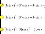
y′ = (ux) ′ = u′ x + u (x) ′ = u′ x + u
Substitute into the original equation.
,
,
,
.
When x ≥ 0
, |x| = x. When x ≤ 0
, |x| = - x . We write |x| = x implying that the top sign refers to values x ≥ 0
, and the lower one - to the values x ≤ 0
.
,
Multiply by dx and divide by .
When u 2 - 1 ≠ 0
we have:
Let's integrate:
Tabular integrals,
.
Let's apply the formula:
(a + b)(a - b) = a 2 - b 2.
Let's put a = u, .
.
Let's take both sides modulo and logarithmize,
.
From here
.
Thus we have:
,
.
We omit the sign of the modulus, since the desired sign is ensured by choosing the sign of the constant C.
Multiply by x and substitute ux = y.
,
.
Square it.
,
,
.
Now consider the case, u 2 - 1 = 0
.
The roots of this equation
.
It is easy to verify that the functions y = x satisfy the original equation.
Answer
,
,
.
References:
N.M. Gunter, R.O. Kuzmin, Collection of problems in higher mathematics, “Lan”, 2003.