Who proposed the map projection. Classifications of cartographic projections. Classification of projections according to the type of normal cartographic grid

3. And finally, the final stage of creating a map is displaying the reduced surface of the ellipsoid on a plane, i.e. the use of map projection (a mathematical way of depicting an ellipsoid on a plane.).

The surface of an ellipsoid cannot be turned onto a plane without distortion. Therefore, it is projected onto a figure that can be deployed onto a plane (Fig). In this case, there are distortions of angles between parallels and meridians, distances, areas.

There are several hundred projections that are used in cartography. Let us further analyze their main types, without going into all the variety of details.

According to the type of distortion, projections are divided into:

1. Equal-angled (conformal) - projections that do not distort angles. At the same time, the similarity of figures is preserved, the scale changes with changes in latitude and longitude. The area ratio is not saved on the map.

2. Equivalent (equivalent) - projections on which the scale of areas is the same everywhere and the areas on the maps are proportional to the corresponding areas on the Earth. However, the length scale at each point is different in different directions. equality of angles and similarity of figures are not preserved.

3. Equidistant projections - projections that maintain a constant scale in one of the main directions.

4. Arbitrary projections - projections that do not belong to any of the considered groups, but have some other properties that are important for practice, are called arbitrary.

Rice. Projection of an ellipsoid onto a figure unfolded into a plane.

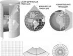
Depending on which figure the ellipsoid surface is projected onto (cylinder, cone or plane), projections are divided into three main types: cylindrical, conical and azimuthal. The type of figure on which the ellipsoid is projected determines the type of parallels and meridians on the map.

Rice. The difference in projections according to the type of figures on which the surface of the ellipsoid is projected and the type of development of these figures on the plane.

In turn, depending on the orientation of the cylinder or cone relative to the ellipsoid, cylindrical and conical projections can be: straight - the axis of the cylinder or cone coincides with the axis of the Earth, transverse - the axis of the cylinder or cone is perpendicular to the axis of the Earth and oblique - the axis of the cylinder or cone is inclined to the axis of the Earth at an angle other than 0° and 90°.

Rice. The difference in projections is the orientation of the figure onto which the ellipsoid is projected relative to the Earth's axis.

The cone and cylinder can either touch the surface of the ellipsoid or intersect it. Depending on this, the projection will be tangent or secant. Rice.

Rice. Tangent and secant projections.

It is easy to see (Fig) that the length of the line on the ellipsoid and the length of the line on the figure that it is projected will be the same along the equator, tangent to the cone for the tangent projection and along the secant lines of the cone and cylinder for the secant projection.

Those. for these lines, the map scale will exactly match the scale of the ellipsoid. For other points on the map, the scale will be slightly larger or smaller. This must be taken into account when cutting map sheets.

The tangent to the cone for the tangent projection and the secant of the cone and cylinder for the secant projection are called standard parallels.

For the azimuthal projection, there are also several varieties.

Depending on the orientation of the plane tangent to the ellipsoid, the azumuthal projection can be polar, equatorial or oblique (Fig)

Rice. Views of the Azimuthal projection by the position of the tangent plane.

Depending on the position of an imaginary light source that projects the ellipsoid onto a plane - in the center of the ellipsoid, at the pole, or at an infinite distance, there are gnomonic (central-perspective), stereographic and orthographic projections.

Rice. Types of azimuthal projection by the position of an imaginary light source.

The geographical coordinates of any point on the ellipsoid remain unchanged for any choice of map projection (determined only by the selected system of "geographical" coordinates). However, along with geographical projections of an ellipsoid on a plane, so-called projected coordinate systems are used. These are rectangular coordinate systems - with the origin at a certain point, most often having coordinates 0,0. Coordinates in such systems are measured in units of length (meters). This will be discussed in more detail below when considering specific projections. Often, when referring to the coordinate system, the words "geographic" and "projected" are omitted, which leads to some confusion. Geographical coordinates are determined by the selected ellipsoid and its bindings to the geoid, "projected" - by the selected projection type after selecting the ellipsoid. Depending on the selected projection, different "projected" coordinates may correspond to one "geographical" coordinates. And vice versa, different “geographic” coordinates can correspond to the same “projected” coordinates if the projection is applied to different ellipsoids. On the maps, both those and other coordinates can be indicated simultaneously, and the “projected” ones are also geographical, if we understand literally that they describe the Earth. We emphasize once again that it is fundamental that the "projected" coordinates are associated with the type of projection and are measured in units of length (meters), while the "geographic" ones do not depend on the selected projection.

Let us now consider in more detail two cartographic projections, the most important for practical work in archeology. These are the Gauss-Kruger projection and the Universal Transverse Mercator (UTM) projection, which are varieties of the conformal transverse cylindrical projection. The projection is named after the French cartographer Mercator, who was the first to use a direct cylindrical projection to create maps.

The first of these projections was developed by the German mathematician Carl Friedrich Gauss in 1820-30. for mapping Germany - the so-called Hanoverian triangulation. As a truly great mathematician, he solved this particular problem in a general way and made a projection suitable for mapping the entire Earth. A mathematical description of the projection was published in 1866. In 1912-19. Another German mathematician, Kruger Johannes Heinrich Louis, conducted a study of this projection and developed a new, more convenient mathematical apparatus for it. Since that time, the projection is called by their names - the Gauss-Kruger projection

The UTM projection was developed after World War II when NATO countries agreed that a standard spatial coordinate system was needed. Since each of the armies of NATO countries used its own spatial coordinate system, it was impossible to accurately coordinate military movements between countries. The definition of UTM system parameters was published by the US Army in 1951.

To obtain a cartographic grid and draw up a map on it in the Gauss-Kruger projection, the surface of the earth's ellipsoid is divided along the meridians into 60 zones of 6 ° each. As you can easily see, this corresponds to dividing the globe into 6° zones when building a map at a scale of 1:100,000. The zones are numbered from west to east, starting from 0°: zone 1 extends from the 0° meridian to the 6° meridian, its central meridian is 3°. Zone 2 - from 6° to 12°, etc. The numbering of nomenclature sheets starts from 180°, for example, sheet N-39 is in the 9th zone.

To link the longitude of the point λ and the number n of the zone in which the point is located, you can use the following relations:

in the Eastern Hemisphere n = (integer of λ/ 6°) + 1, where λ are degrees east

in the Western Hemisphere, n = (integer of (360-λ)/ 6°) + 1, where λ are degrees west.

Rice. Partitioning into zones in the Gauss-Kruger projection.

Further, each of the zones is projected onto the surface of the cylinder, and the cylinder is cut along the generatrix and unfolded onto a plane. Rice

Rice. Coordinate system within 6 degree zones in GC and UTM projections.

In the Gauss-Kruger projection, the cylinder touches the ellipsoid along the central meridian and the scale along it is equal to 1. Fig.

For each zone, the coordinates X, Y are measured in meters from the origin of the zone, and X is the distance from the equator (vertically!), And Y is the horizontal distance. The vertical grid lines are parallel to the central meridian. The origin of coordinates is shifted from the central meridian of the zone to the west (or the center of the zone is shifted to the east, the English term “false easting” is often used to denote this shift) by 500,000 m so that the X coordinate is positive in the entire zone, i.e. the X coordinate on the central meridian is 500,000 m.

In the southern hemisphere, a northing offset (false northing) of 10,000,000 m is introduced for the same purposes.

The coordinates are written as X=1111111.1 m, Y=6222222.2 m or

X s =1111111.0 m, Y=6222222.2 m

X s - means that the point is in the southern hemisphere

6 - the first or two first digits in the Y coordinate (respectively, only 7 or 8 digits before the decimal point) indicate the zone number. (St. Petersburg, Pulkovo -30 degrees 19 minutes east longitude 30:6 + 1 = 6 - zone 6).

All topographic maps of the USSR at a scale of 1:500,000 were compiled in the Gauss-Kruger projection for the Krasovsky ellipsoid, and the larger application of this projection in the USSR began in 1928.

2. The UTM projection is generally similar to the Gauss-Kruger projection, but the 6-degree zones are numbered differently. The zones are counted from the 180th meridian to the east, so the zone number in the UTM projection is 30 more than the Gauss-Kruger coordinate system (St. zone).

In addition, UTM is a projection onto a secant cylinder and the scale is equal to one along two secant lines that are 180,000 m from the central meridian.

In the UTM projection, the coordinates are given as: Northern Hemisphere, zone 36, N (northern position)=1111111.1 m, E (eastern position)=222222.2 m. The origin of each zone is also shifted 500,000 m west of the central meridian and 10,000,000 m south of the equator for the southern hemisphere.

Modern maps of many European countries have been compiled in the UTM projection.

Comparison of Gauss-Kruger and UTM projections is given in the table

Parameter	UTM	Gaus-Kruger
Zone size	6 degrees	6 degrees
Prime Meridian	-180 degrees	0 degrees (GMT)
Scale factor = 1	Crossing at a distance of 180 km from the central meridian of the zone	Central meridian of the zone.
Central meridian and its corresponding zone	3-9-15-21-27-33-39-45 etc. 31-32-33-34-35-35-37-38-…	3-9-15-21-27-33-39-45 etc. 1-2-3-4-5-6-7-8-…
Corresponding to the center of the meridian zone	31 32 33 34
Scale factor along the central meridian	0,9996
False east (m)	500 000	500 000
False north (m)	0 - northern hemisphere	0 - northern hemisphere
		10,000,000 - southern hemisphere

Looking ahead, it should be noted that most GPS navigators can show coordinates in the UTM projection, but cannot in the Gauss-Kruger projection for the Krasovsky ellipsoid (ie, in the SK-42 coordinate system).

Each sheet of a map or plan has a finished design. The main elements of the sheet are: 1) the actual cartographic image of a section of the earth's surface, the coordinate grid; 2) sheet frame, the elements of which are determined by the mathematical basis; 3) framing (auxiliary equipment), which includes data facilitating the use of the card.

The cartographic image of the sheet is limited to the inner frame in the form of a thin line. The northern and southern sides of the frame are segments of parallels, the eastern and western sides are segments of meridians, the value of which is determined by the general system of marking topographic maps. The values of the longitude of the meridians and the latitude of the parallels that bound the map sheet are signed near the corners of the frame: longitude on the continuation of the meridians, latitude on the continuation of the parallels.

At some distance from the inner frame, the so-called minute frame is drawn, which shows the outlets of the meridians and parallels. The frame is a double line drawn into segments corresponding to the linear extent of 1 "meridian or parallel. The number of minute segments on the northern and southern sides of the frame is equal to the difference in the longitude values of the western and eastern sides. On the western and eastern sides of the frame, the number of segments is determined by the difference in the latitude values of the northern and south sides.

The final element is the outer frame in the form of a thickened line. Often it is integral with the minute frame. In the intervals between them, the marking of minute segments into ten-second segments is given, the boundaries of which are marked with dots. This makes the map easier to work with.

On maps of scale 1: 500,000 and 1: 1,000,000, a cartographic grid of parallels and meridians is given, and on maps of scale 1: 10,000 - 1: 200,000 - a coordinate grid, or kilometer, since its lines are drawn through an integer number of kilometers ( 1 km on a scale of 1:10,000 - 1:50,000, 2 km on a scale of 1:100,000, 4 km on a scale of 1:200,000).

The values of the kilometer lines are signed in the intervals between the inner and minute frames: abscissas at the ends of the horizontal lines, ordinates at the ends of the vertical ones. At the extreme lines, the full values of the coordinates are indicated, at the intermediate ones - abbreviated ones (only tens and units of kilometers). In addition to the designations at the ends, some of the kilometer lines have signatures of coordinates inside the sheet.

An important element of the marginal design is information about the average magnetic declination for the territory of the map sheet, related to the moment of its determination, and the annual change in magnetic declination, which is placed on topographic maps at a scale of 1: 200,000 and larger. As you know, the magnetic and geographic poles do not coincide and the arrow of the commas shows a direction slightly different from the direction to the geographic zone. The magnitude of this deviation is called the magnetic declination. It can be east or west. By adding to the value of the magnetic declination the annual change in the magnetic declination, multiplied by the number of years that have passed since the creation of the map until the current moment, determine the magnetic declination at the current moment.

In concluding the topic on the basics of cartography, let us briefly dwell on the history of cartography in Russia.

The first maps with a displayed geographical coordinate system (maps of Russia by F. Godunov (published in 1613), G. Gerits, I. Massa, N. Witsen) appeared in the 17th century.

In accordance with the legislative act of the Russian government (the boyar "verdict") of January 10, 1696 "On the removal of a drawing of Siberia on canvas with an indication of cities, villages, peoples and distances between tracts" S.U. Remizov (1642-1720) created a huge (217x277 cm) cartographic work "Drawing of all Siberian cities and lands", which is now in the permanent exhibition of the State Hermitage. 1701 - January 1 - the date on the first title page of Remizov's Atlas of Russia.

In 1726-34. the first Atlas of the All-Russian Empire is published, the head of the work on the creation of which was the chief secretary of the Senate I.K. Kirillov. The atlas was published in Latin, and consisted of 14 special and one general maps under the title "Atlas Imperii Russici". In 1745 the All-Russian Atlas was published. Initially, the work on compiling the atlas was led by academician, astronomer I. N. Delil, who in 1728 presented a project for compiling an atlas of the Russian Empire. Starting from 1739, the work on compiling the atlas was carried out by the Geographical Department of the Academy of Sciences, established on the initiative of Delisle, whose task was to compile maps of Russia. Delisle's atlas includes comments on maps, a table with the geographical coordinates of 62 Russian cities, a map legend and the maps themselves: European Russia on 13 sheets at a scale of 34 versts per inch (1:1428000), Asian Russia on 6 sheets on a smaller scale and a map of all of Russia on 2 sheets on a scale of about 206 versts per inch (1:8700000) The Atlas was published in the form of a book in parallel editions in Russian and Latin with the application of the General Map.

When creating the Delisle atlas, much attention was paid to the mathematical basis of the maps. For the first time in Russia, an astronomical determination of the coordinates of strong points was carried out. The table with coordinates indicates the way they were determined - "for reliable reasons" or "when compiling a map" During the 18th century, a total of 67 complete astronomical determinations of coordinates were made relating to the most important cities of Russia, and 118 determinations of points in latitude were also made . On the territory of Crimea, 3 points were identified.

From the second half of the XVIII century. the role of the main cartographic and geodetic institution of Russia gradually began to be performed by the Military Department

In 1763 a Special General Staff was created. Several dozen officers were selected there, who officers were sent to remove the areas where the troops were located, the routes of their possible following, the roads along which messages passed by military units. In fact, these officers were the first Russian military topographers who completed the initial scope of work on mapping the country.

In 1797, the Card Depot was established. In December 1798, the Depot received the right to control all topographic and cartographic work in the empire, and in 1800 the Geographical Department was attached to it. All this made the Map Depot the central cartographic institution of the country. In 1810 the Kart Depot was taken over by the Ministry of War.

February 8 (January 27, old style) 1812, when the highest approved "Regulations for the Military Topographic Depot" (hereinafter VTD), which included the Map Depot as a special department - the archive of the military topographic depot. By order of the Minister of Defense of the Russian Federation of November 9, 2003, the date of the annual holiday of the VTU of the General Staff of the Armed Forces of the Russian Federation was set - February 8.

In May 1816, the VTD was included in the General Staff, while the head of the General Staff was appointed director of the VTD. Since this year, the VTD (regardless of renaming) has been permanently part of the Main or General Staff. VTD led the Corps of Topographers, created in 1822 (after 1866, the Corps of Military Topographers)

The most important results of the work of the VTD for almost a whole century after its creation are three large maps. The first is a special map of European Russia on 158 sheets, 25x19 inches in size, on a scale of 10 versts in one inch (1:420000). The second is a military topographic map of European Russia on a scale of 3 versts per inch (1:126000), the projection of the map is conical of Bonn, longitude is calculated from Pulkovo.

The third is a map of Asian Russia on 8 sheets 26x19 inches in size, on a scale of 100 versts per inch (1:42000000). In addition, for part of Russia, especially for the border regions, maps were prepared on a half-verst (1:21000) and verst (1:42000) scale (on the Bessel ellipsoid and the Müfling projection).

In 1918, the Military Topographic Directorate (the assignee of the VTD) was introduced into the structure of the All-Russian General Staff, which later, until 1940, took on different names. The corps of military topographers is also subordinate to this department. From 1940 to the present, it has been called the "Military Topographic Directorate of the General Staff of the Armed Forces."

In 1923, the Corps of Military Topographers was transformed into a military topographic service.

In 1991, the Military Topographic Service of the Armed Forces of Russia was formed, which in 2010 was transformed into the Topographic Service of the Armed Forces of the Russian Federation.

It should also be said about the possibility of using topographic maps in historical research. We will only talk about topographic maps created in the 17th century and later, the construction of which was based on mathematical laws and a specially conducted systematic survey of the territory.

General topographic maps reflect the physical state of the area and its toponymy at the time the map was compiled.

Maps of small scales (more than 5 versts in an inch - smaller than 1:200000) can be used to localize the objects indicated on them, only with a large uncertainty in coordinates. The value of the information contained is in the possibility of identifying changes in the toponymy of the territory, mainly while preserving it. Indeed, the absence of a toponym on a later map may indicate the disappearance of an object, a change in name, or simply its erroneous designation, while its presence will confirm an older map, and, as a rule, in such cases more accurate localization is possible..

Maps of large scales provide the most complete information about the territory. They can be directly used to search for objects marked on them and preserved to this day. The ruins of buildings are one of the elements included in the legend of topographic maps, and although only a few of the ruins indicated are archaeological monuments, their identification is a matter worthy of consideration.

The coordinates of the surviving objects, determined from topographic maps of the USSR, or by direct measurements using the global space positioning system (GPS), can be used to link old maps to modern coordinate systems. However, even maps of the early-mid 19th century can contain significant distortions in the proportions of the terrain in certain areas of the territory, and the procedure for linking maps consists not only of correlating the origins of coordinates, but also requires uneven stretching or compression of individual sections of the map, which is carried out on the basis of knowing the coordinates of a large number of reference points. points (the so-called map image transformation).

After the binding, it is possible to compare the signs on the map with the objects present on the ground at the present time, or that existed in the periods preceding or following the time of its creation. To do this, it is necessary to compare the available maps of different periods and scales.

Large-scale topographic maps of the 19th century seem to be very useful when working with boundary plans of the 18th-19th centuries, as a link between these plans and large-scale maps of the USSR. Boundary plans were drawn up in many cases without substantiation at strong points, with an orientation along the magnetic meridian. Due to changes in the nature of the terrain caused by natural factors and human activity, a direct comparison of boundary and other detailed plans of the last century and maps of the 20th century is not always possible, however, a comparison of the detailed plans of the last century with a modern topographic map seems to be easier.

Another interesting possibility of using large-scale maps is their use to study changes in the contours of the coast. Over the past 2.5 thousand years, the level of, for example, the Black Sea has risen by at least a few meters. Even in the two centuries that have passed since the creation of the first maps of the Crimea in the VTD, the position of the coastline in a number of places could have shifted by a distance of several tens to hundreds of meters, mainly due to abrasion. Such changes are quite commensurate with the size of fairly large settlements by ancient standards. Identification of areas of the territory absorbed by the sea can contribute to the discovery of new archaeological sites.

Naturally, the three-verst and verst maps can serve as the main sources for the territory of the Russian Empire for these purposes. The use of geoinformation technologies makes it possible to overlay and link them to modern maps, to combine layers of large-scale topographic maps of different times, and then split them into plans. Moreover, the plans created now, like the plans of the 20th century, will be tied to the plans of the 19th century.

Modern values of the Earth's parameters: Equatorial radius, 6378 km. Polar radius, 6357 km. The average radius of the Earth, 6371 km. Equator length, 40076 km. Meridian length, 40008 km...

Here, of course, it must be taken into account that the value of the “stage” itself is a debatable issue.

A diopter is a device that serves to direct (sight) a known part of a goniometric instrument to a given object. The guided part is usually supplied with two D. - eye, with a narrow slot, and subject, with a wide slit and a hair stretched in the middle (http://www.wikiznanie.ru/ru-wz/index.php/Diopter).

Based on materials from the site http://ru.wikipedia.org/wiki/Soviet _engraving_system_and_nomenclature_of_topographic_maps#cite_note-1

Gerhard Mercator (1512 - 1594) - the Latinized name of Gerard Kremer (both Latin and Germanic surnames mean "merchant"), a Flemish cartographer and geographer.

The description of the marginal design is given in the work: "Topography with the basics of geodesy." Ed. A.S. Kharchenko and A.P. Bozhok. M - 1986

Since 1938, for 30 years, the VTU (under Stalin, Malenkov, Khrushchev, Brezhnev) was headed by General M.K. Kudryavtsev. No one has held such a position in any army in the world for such a long time.

LECTURE №4

MAP PROJECTIONS

Kartographic projections called mathematical methods of image on the plane of the surface of the earth's ellipsoid or ball. The image of the degree grid of the Earth on the map is called the cartographic grid, and the intersection points of the meridians and parallels are the nodal points.

The construction of maps includes first an image on a plane (paper) of a cartographic grid, and then filling the cells of the grid with contours and other designations of geographical objects. Meshing can be done in various ways. So, when applying perspective projections the cartographic grid is obtained, as it were, by projecting nodal points from the surface of a ball onto a plane (Fig. 4) or onto another geometric surface (cone, cylinder), which then unfolds into a plane without distortion. An example of the practical construction of a map grid of the northern hemisphere in a perspective way is shown in Figure 4.

The picture plane P here touches the surface of the northern hemisphere at the point of the North Pole. Rectilinear projecting rays from the center K are the nodal points of intersection of the meridian with the equator and the parallels of 30 ° and 60 ° latitude are transferred to the picture plane. Thus, the radii of these parallels on the plane are determined. Meridians are depicted on a plane by straight lines emanating from the pole point and spaced from each other at equal angles. The figure shows half of the grid. The second half is easy to mentally imagine, and, if necessary, build.

Building a map using perspective projections does not require the use of higher mathematics, so they began to be used long before its development, from ancient times. Nowadays, in cartographic production, maps are built unpromising methodmi- by calculating the position of the nodal points of the cartographic grid on the plane. The calculation is performed by solving a system of equations relating the latitude and longitude of nodal points with their rectangular coordinates X and Y on surface. The equations involved are quite complex. An example of relatively simple formulas can be the following:

X=R ´ sin j

Y= R´ cos j-sinl .

In these equations R- radius (average) of the Earth, rounded off as 6370 km, and j, l- geographic coordinates of nodal points.

Classification of map projections

The projections used for the construction of geographical maps can be grouped according to different classification criteria, of which the main ones are: a) the type of "auxiliary surface" and its orientation, b) the nature of the distortions.

Classification of cartographic projections by type of auxiliarybody surface and its orientation. Cartographic grids of maps are obtained in modern production in an analytical way. However, in the names of the projections, the terms “cylindrical”, “conical” and others are traditionally preserved, corresponding to the methods of geometric constructions that were used in the past to build grids) The use of these terms in explaining these terms will help to understand the features of the cartographic grids obtained on their basis. Currently, this classification feature is treated as a type of normal cartographic grid

Cylindrical projections. When constructing cylindrical projections, they imagine that the nodal points, and hence the lines of the degree network, are projected from the spherical surface of the globe to the side surface of the cylinder, the axis of which coincides with the axis of the globe, and the diameters of both bodies are equal (Fig. 5). Using a tangent cylinder as an auxiliary surface, it is taken into account that the nodal points of the equator are A, B, C,D and others are both on the globe and on the cylinder. Other nodal points are transferred from the globe to the surface of the cylinder. Yes, dots E and F, located on the same meridian with point C, are transferred to points £ "and F\ In this case, they will be located on the cylinder on a straight line perpendicular to the equator line. This determines the shape of the meridians in this projection. Parallels to the surface of the cylinder are projected in the form of circles parallel to the equator line (for example, the parallel in which the points are located F[ and e").

When the surface of the cylinder is turned into a plane, all the lines of the cartographic grid turn out to be straight, the meridians are perpendicular to the parallels and spaced at equal distances from each other. This is the general view of the cartographic grid built using a cylinder tangent to the globe and having a common axis with it.

For such cylindrical projections, the equator serves as the line of zero distortion, and the isocoles have the form of straight lines parallel to the equator; the main directions coincide with the lines of the cartographic grid, while the distance from the equator increases the distortion.

In these projections, projection is also used for cylinders with a diameter smaller than the diameter of the globe, and located differently relative to the globe. Depending on the orientation of the cylinder, the resulting cartographic grids (as well as the projections themselves) are called normal, oblique, or transverse. Normal Cylindrical Grids build on cylinders whose axes coincide with the axis of the globe; oblique- on cylinders, the axis of which makes an acute angle with the axis of the globe; cross grids formed by a cylinder whose axis is at right angles to the axis of the globe .

A normal cylindrical mapping grid on a tangent cylinder has a zero distortion line at the equator. The normal grid on the secant cylinder has two zero distortion lines located along the parallels of the section of the cylinder with the globe (with latitudes j1 and j2). In this case, due to the compression of the grid area between the lines of zero distortion, the length scales along the parallels are here less than the main one; to the outer side of the lines of zero distortion, they are larger than the main scale - as a result of stretching the parallels when designing from a globe to a cylinder.

The oblique cylindrical grid on the secant cylinder has a line of zero distortions in the northern part in the form of a straight line perpendicular to the middle meridian of the map and tangent to the parallel with latitude j; the appearance of the grid is represented by curved lines of meridians and parallels.

An example of a transverse cylindrical projection is the Gauss-Kruger projection, in which each transverse cylinder is used to project the surface of one Gaussian zone.

conical projections. To build cartographic grids in conic projections, normal cones are used - tangent or secant.

fig.6

fig.7

Everyone has normal conic projections the appearance of the cartographic grid is specific: meridians are straight lines converging at a point depicting the top of a cone on a plane, parallels are arcs of concentric circles with a center at the vanishing point of the meridians. Meshes built on tangent cones have one line of zero distortion, with the distance from which the distortion increases (Fig. 6). Their isocoles have the form of arcs of circles coinciding with parallels. Grids built on a secant cone (Fig. 6b) have the same appearance, but a different distribution of distortion: they have two lines of zero distortion. Between them, partial scales along the parallels are smaller than the main scale, and on the outer sections of the grid - larger than the main scale. The main directions of all normal conical grids coincide with meridians and parallels.

Azimuthal projections. Azimuthal grids are called cartographic grids, which are obtained by projecting a degree grid of a globe onto a tangent plane (Fig.). normal azimutated mesh obtained as a result of transfer to a plane tangent to the globe at the pole point (Fig. 7 A), transversenuyu- when touching the plane at the point of the equator (Fig. 7, B) and toSuyu- when transferred to a differently oriented plane (Fig. 7, V). The appearance of the grids is clearly visible in Figure 7.

All azimuthal grids have the following general properties regarding distortion: the point of zero distortion (ZDT) is the point of contact between the globe and the plane (usually it is located in the center of the map); the magnitude of the distortions increases with distance in all directions from the HPS, so the isocoles of the azimuthal projections have the shape of concentric circles with the center at the HPS. The principal directions follow the radius and the lines perpendicular to them. The name of this group of projections is due to the fact that on the cartographic grid built in the azimuthal projection, at the former point of contact between the globe and the plane (i.e., at the point of zero distortion), the azimuths of all directions are not distorted

Polyconic projections. The construction of a grid in a polyconical projection can be represented by projecting segments of the globe's degree grid onto the surface of several tangent cones and then sweeping the stripes formed on the surface of the cones into the plane. The general principle of such a design is shown in Figure 8. The letters in Figure 8, A indicate the tops of the cones. For each, a latitudinal section of the globe surface is projected adjacent to the parallel of contact of the corresponding cone. After scanning the cones, these sections are imaged as stripes on a plane; the stripes touch along the middle meridian of the map . The final form of the grid is obtained after the elimination of gaps between the strips by stretching.

fig.8

For the appearance of cartographic grids in a polyconic projection, it is characteristic that the meridians have the form of curved lines (except for the middle one - straight), and the parallels are arcs of eccentric circles. In polyconic projections used to build world maps, the equatorial section is projected onto a tangent cylinder, therefore, on the resulting grid, the equator has the form of a straight line perpendicular to the middle meridian.

Map grids in polyconic projections have length scales close to the main ones in equatorial areas. Along the meridians and parallels, they are enlarged compared to the main scale, which is especially noticeable in the peripheral parts. Accordingly, in these parts, the areas are also significantly distorted.

Conditional projections. Conditional projections include such projections in which the form of the resulting cartographic grids cannot be represented on the basis of projection onto some auxiliary surface. They are often obtained analytically (based on solving systems of equations). This is a very large group of projections. Of these, they are distinguished according to the features of the appearance of the cartographic grid pseudocylindrical projections (Fig. 9). As can be seen from the figure, for pseudocylindrical projections, the equator and parallels are straight lines parallel to each other (which makes them similar to cylindrical projections), and their meridians are curved lines.

Fig.9

View of distortion ellipses in projections of equal area - A, equiangular - B, arbitrary - B, including equidistant along the meridian - G and equidistant along the parallel - D. The diagrams show the distortion of the angle 45 °

Map projections are distinguished by the nature of the distortions and by construction. By the nature of the distortions, projections are distinguished:

1) Equangular, preserving the magnitude of the angles, here a=b. Distortion ellipses look like circles of different areas.

2) Equal-sized, preserving the areas of objects. In them R=mn cos e=l; therefore, increasing the scale of lengths along the parallels causes a decrease in the scale of lengths along the meridians and distortion of angles and shapes.

3) Arbitrary, distorting angles and areas. Among them, a group of equidistant projections stands out, in which the main scale in one of the main directions is preserved.

Of great practical importance is the division of projections by territorial coverage into projections for maps of the world, hemispheres, continents and oceans, states and their parts.

Below are tables of external signs of widespread projections for different territories, compiled.

table 1

Table for determining the cartographic grids of maps of the Eastern and Western hemispheres

How do the intervals change according to: Middle meridian and equator Meridian and equator from the center to the edges of the hemisphere	What lines represent parallels	Name of projections
Decreases from 1 to approximately 0.7	Curves that increase curvature with distance from the middle meridian to the extreme	Equal area equatorial azimuthal Lambert
Decreases from 1 to approximately 0.8	Equatorial azimuthal Ginzburg
Increase from 1 to approximately 2	Arcs of circles	Equatorial stereographic
greatly reduced		Equatorial orthographic

table 2

Table for determining projections of cartographic grids of world maps

Frame shape, map or whole grid view	What lines represent parallels and meridians	How do the intervals along the middle meridian change with distance from the equator	Projection Name
Rectangle frame	Parallels-straight lines, meridians-curves	Increase between parallels 70 and 80° is almost 1.5 times greater than between the equator and parallel 10 °	Pseudocylindrical projection of TsNIIGAiK
Grid and Rectangle Frame	Parallels and meridians - straight lines	Increase strongly: between the parallels of 60 and 80 ° approximately 3 times more than between the equator and the parallel of 20 °	Cylindrical Mercator
Grid and Rectangle Frame	Meridian parallels - straight lines	Increasing: parallels approximately 2 2/3 times more than between the equator and parallel 20°	Cylindrical Urmaeva

The definition of map projections of geographical maps is determined using tables and calculations. First of all, they find out which territory is shown on the analyzed map and which table should be used when determining the projection. Then the type of parallels and meridians and the nature of the gaps between the parallels along the direct meridian are determined. The nature of the meridians is also determined: whether they are straight or only the middle meridian is straight, and the rest are curves, symmetrical with respect to the middle one. The straightness of the meridians is checked with a ruler. If the meridians turned out to be straight, specify whether they are parallel to each other. When considering parallels, find out whether the parallels are arcs of circles, curves or straight lines. This is established by comparing the sag arrows for arcs of equal chords: with equal sag arrows, the lines are arcs of circles, with unequal sag arrows, the parallels are complex curves . To determine the nature of the curvature of the line, you can also do the following. Three points of this curve are marked on a sheet of tracing paper. If, when moving the leaf along the line, all three points coincide with the curve, then this curve will be an arc of a circle. If the parallels turn out to be arcs, their concentricity should be checked, for which the distances between adjacent parallels in the middle of the map and on the edge are measured. If these distances are constant, the arcs are concentric.

Both direct conic and azimuthal polar projections have rectilinear meridians diverging from one point. A section of the direct conic grid can be distinguished from a section of the polar azimuth projection grid by measuring the angle between two meridians spaced 60-90° apart. If this angle turned out to be less than the corresponding difference in longitudes, signed on the map, then this is a conic projection, if it is equal to the difference in longitudes, it is azimuthal.

Determining the average distortion sizes for geographic objects can be done in two ways:

1) by measuring segments of meridians and parallels on the map and subsequent calculations using formulas;

2) according to maps with isocols.

In the first case, the partial scales are first calculated along the meridians (T) and parallels \(P) and express them in fractions of the main scale:

where - l1 the length of the meridian arc on the map, L1 - the length of the meridian arc on the ellipsoid, l2 - the length of the parallel arc on the map, L2 - arc length of the parallel on the ellipsoid { L1 and L2 taken from application tables; M- the denominator of the main scale.

Then they measure on the map with a protractor the angle e between the tangents to the parallel and the meridian at a given point; determine the deviation of the angle q from 90°; e = q -90°.

Based on known formulas, the distortion values are calculated R,a, b, w, To.

In the second case, isocol maps are used. From these maps, values are taken for 2-3 points of objects with an accuracy allowed by visual interpolation, then it is possible to establish which group this projection belongs to by the nature of distortions.

In the transition from the physical surface of the Earth to its display on a plane (on a map), two operations are performed: projecting the earth's surface with its complex relief onto the surface of an earth ellipsoid, the dimensions of which are established by means of geodetic and astronomical measurements, and the image of the ellipsoid surface on a plane by means of one of the cartographic projections.
A map projection is a specific way of displaying the surface of an ellipsoid on a plane.
The display of the earth's surface on a plane is carried out in various ways. The simplest one is perspective . Its essence lies in projecting an image from the surface of the Earth model (globe, ellipsoid) onto the surface of a cylinder or cone, followed by a turn into a plane (cylindrical, conical) or direct projection of a spherical image onto a plane (azimuth).
One easy way to understand how map projections change spatial properties is to visualize the projection of light through the Earth onto a surface called a projection surface.
Imagine that the surface of the Earth is transparent and has a map grid on it. Wrap a piece of paper around the earth. A light source at the center of the earth will cast shadows from the grid onto the piece of paper. You can now unfold the paper and lay it flat. The shape of the coordinate grid on a flat surface of paper is very different from its shape on the surface of the Earth (Fig. 5.1).

Rice. 5.1. Geographic coordinate system grid projected onto a cylindrical surface

The map projection distorted the cartographic grid; objects near the pole are elongated.
Building in a perspective way does not require the use of the laws of mathematics. Please note that in modern cartography, cartographic grids are built analytical (mathematical) way. Its essence lies in the calculation of the position of nodal points (points of intersection of meridians and parallels) of the cartographic grid. The calculation is performed on the basis of solving a system of equations that relate the geographic latitude and geographic longitude of nodal points ( φ, λ ) with their rectangular coordinates ( x, y) on surface. This dependence can be expressed by two equations of the form:

x = f 1 (φ, λ); (5.1)
y = f 2 (φ, λ), (5.2)

called map projection equations. They allow you to calculate rectangular coordinates x, y displayed point by geographic coordinates φ and λ . The number of possible functional dependencies and, therefore, projections is unlimited. It is only necessary that each point φ , λ the ellipsoid was depicted on the plane by a uniquely corresponding point x, y and that the image is continuous.

5.2. DISTORTION

Decomposing a spheroid onto a plane is no easier than flattening a piece of watermelon peel. When going to a plane, as a rule, angles, areas, shapes and lengths of lines are distorted, so for specific purposes it is possible to create projections that will significantly reduce any one type of distortion, for example, areas. Cartographic distortion is a violation of the geometric properties of sections of the earth's surface and objects located on them when they are depicted on a plane. .
Distortions of all kinds are closely related. They are in such a relationship that a decrease in one type of distortion immediately leads to an increase in another. As area distortion decreases, angle distortion increases, and so on. Rice. Figure 5.2 shows how 3D objects are compressed to fit on a flat surface.

Rice. 5.2. Projecting a spherical surface onto a projection surface

On different maps, distortions can be of different sizes: on large-scale maps they are almost imperceptible, but on small-scale maps they can be very large.
In the middle of the 19th century, the French scientist Nicolas August Tissot gave a general theory of distortions. In his work, he proposed to use special distortion ellipses, which are infinitesimal ellipses at any point on the map, representing infinitesimal circles at the corresponding point on the surface of the earth's ellipsoid or globe. The ellipse becomes a circle at the zero distortion point. Changing the shape of the ellipse reflects the degree of distortion of angles and distances, and the size - the degree of distortion of areas.

Rice. 5.3. Ellipse on the map ( a) and the corresponding circle on the globe ( b)

The distortion ellipse on the map can take a different position relative to the meridian passing through its center. The orientation of the distortion ellipse on the map is usually determined by azimuth of its semi-major axis . The angle between the north direction of the meridian passing through the center of the distortion ellipse and its nearest semi-major axis is called the orientation angle of the distortion ellipse. On fig. 5.3, a this corner is marked with the letter A 0 , and the corresponding angle on the globe α 0 (Fig. 5.3, b).
Azimuths of any direction on the map and on the globe are always measured from the north direction of the meridian in a clockwise direction and can have values from 0 to 360°.
Any arbitrary direction ( OK) on a map or on a globe ( O 0 TO 0 ) can be determined either by the azimuth of a given direction ( A- on the map, α - on the globe) or the angle between the semi-major axis closest to the northern direction of the meridian and the given direction ( v- on the map, u- on the globe).

5.2.1. Length distortion

Length distortion - basic distortion. The rest of the distortions follow logically from it. Length distortion means the inconsistency of the scale of a flat image, which manifests itself in a change in scale from point to point, and even at the same point, depending on the direction.
This means that there are 2 types of scale on the map:

main scale (M);
private scale .

main scale maps call the degree of general reduction of the globe to a certain size of the globe, from which the earth's surface is transferred to the plane. It allows you to judge the decrease in the length of the segments when they are transferred from the globe to the globe. The main scale is written under the southern frame of the map, but this does not mean that the segment measured anywhere on the map will correspond to the distance on the earth's surface.
The scale at a given point on the map in a given direction is called private . It is defined as the ratio of an infinitesimal segment on a map dl TO to the corresponding segment on the surface of the ellipsoid dl W . The ratio of the private scale to the main one, denoted by μ , characterizes the distortion of lengths

(5.3)

To assess the deviation of a particular scale from the main one, use the concept zoom in (WITH) defined by the relation

(5.4)

From formula (5.4) it follows that:

at WITH= 1 the partial scale is equal to the main scale ( µ = M), i.e., there are no length distortions at a given point of the map in a given direction;
at WITH> 1 partial scale larger than the main one ( µ > M);
at WITH < 1 частный масштаб мельче главного (µ < М ).

For example, if the main scale of the map is 1: 1,000,000, zoom in WITH equals 1.2, then µ \u003d 1.2 / 1,000,000 \u003d 1/833,333, i.e. one centimeter on the map corresponds to approximately 8.3 km on the ground. The private scale is larger than the main one (the value of the fraction is larger).
When depicting the surface of a globe on a plane, the partial scales will be numerically larger or smaller than the main scale. If we take the main scale equal to one ( M= 1), then the partial scales will be numerically greater or less than unity. In this case under the private scale, numerically equal to the scale increase, one should understand the ratio of an infinitesimal segment at a given point on the map in a given direction to the corresponding infinitesimal segment on the globe:

(5.5)

Partial Scale Deviation (µ )from unity determines the length distortion at a given point on the map in a given direction ( V):

V = µ - 1 (5.6)

Often the length distortion is expressed as a percentage of unity, i.e., to the main scale, and is called relative length distortion :

q = 100(µ - 1) = V×100(5.7)

For example, when µ = 1.2 length distortion V= +0.2 or relative length distortion V= +20%. This means that a segment of length 1 cm, taken on the globe, will be displayed on the map as a segment of length 1.2 cm.
It is convenient to judge the presence of length distortion on the map by comparing the size of the meridian segments between adjacent parallels. If they are everywhere equal, then there is no distortion of the lengths along the meridians, if there is no such equality (Fig. 5.5 segments AB and CD), then there is a distortion of the line lengths.

Rice. 5.4. Part of a map of the Eastern Hemisphere showing cartographic distortions

If a map depicts such a large area that it shows both the equator 0º and the parallel 60° of latitude, then it is not difficult to determine from it whether there is a distortion of lengths along the parallels. To do this, it is enough to compare the length of the segments of the equator and parallels with a latitude of 60 ° between adjacent meridians. It is known that the parallel of 60° latitude is two times shorter than the equator. If the ratio of the indicated segments on the map is the same, then there is no distortion of the lengths along the parallels; otherwise, it exists.
The largest indicator of length distortion at a given point (the major semi-axis of the distortion ellipse) is denoted by the Latin letter a, and the smallest one (semi-minor axis of the distortion ellipse) - b. Mutually perpendicular directions in which the largest and smallest indicators of length distortion act, called the main directions .
To assess various distortions on maps, of all partial scales, partial scales in two directions are of greatest importance: along meridians and along parallels. private scale along the meridian usually denoted by the letter m , and the private scale parallel - letter n.
Within the limits of small-scale maps of relatively small territories (for example, Ukraine), the deviations of the length scales from the scale indicated on the map are small. Errors in measuring lengths in this case do not exceed 2 - 2.5% of the measured length, and they can be neglected when working with school maps. Some maps for approximate measurements are accompanied by a measuring scale, accompanied by explanatory text.
On the nautical charts , built in the Mercator projection and on which the loxodrome is depicted by a straight line, no special linear scale is given. Its role is played by the eastern and western frames of the map, which are meridians divided into divisions through 1′ in latitude.
In maritime navigation, distances are measured in nautical miles. Nautical mile is the average length of the meridian arc of 1′ in latitude. It contains 1852 m. Thus, the frames of the sea chart are actually divided into segments equal to one nautical mile. By determining in a straight line the distance between two points on the map in minutes of the meridian, the actual distance in nautical miles along the loxodrome is obtained.

Figure 5.5. Measuring distances on a sea chart.

5.2.2. Corner distortion

Angular distortions follow logically from length distortions. The angle difference between the directions on the map and the corresponding directions on the surface of the ellipsoid is taken as a characteristic of the distortion of the angles on the map.
For angle distortion between the lines of the cartographic grid, they take the value of their deviation from 90 ° and designate it with a Greek letter ε (epsilon).
ε = Ө - 90°, (5.8)
where in Ө (theta) - the angle measured on the map between the meridian and the parallel.

Figure 5.4 indicates that the angle Ө is equal to 115°, therefore, ε = 25°.
At a point where the angle of intersection of the meridian and the parallel remains right on the chart, the angles between other directions can be changed on the chart, since at any given point the amount of angle distortion can change with direction.
For the general indicator of the distortion of angles ω (omega), the greatest distortion of the angle at a given point is taken, equal to the difference between its magnitude on the map and on the surface of the earth's ellipsoid (ball). When known x indicators a and b value ω determined by the formula:

(5.9)

5.2.3. Area distortion

Area distortions follow logically from length distortions. The deviation of the area of the distortion ellipse from the original area on the ellipsoid is taken as a characteristic of the area distortion.
A simple way to identify the distortion of this type is to compare the areas of the cells of the cartographic grid, limited by parallels of the same name: if the areas of the cells are equal, there is no distortion. This takes place, in particular, on the map of the hemisphere (Fig. 4.4), on which the shaded cells differ in shape, but have the same area.
Area Distortion Index (R) is calculated as the product of the largest and smallest indicators of length distortion at a given location on the map
p = a×b (5.10)
The main directions at a given point on the map may coincide with the lines of the cartographic grid, but may not coincide with them. Then the indicators a and b according to famous m and n calculated according to the formulas:

(5.11)
(5.12)

The distortion factor included in the equations R recognize in this case by the product:

p = m×n×cos ε, (5.13)

Where ε (epsilon) - the deviation of the angle of intersection of the cartographic grid from 9 0°.

5.2.4. Form distortion

Shape distortion consists in the fact that the shape of the site or the territory occupied by the object on the map is different from their shape on the level surface of the Earth. The presence of this type of distortion on the map can be established by comparing the shape of the cartographic grid cells located at the same latitude: if they are the same, then there is no distortion. In figure 5.4, two shaded cells with a difference in shape indicate the presence of a distortion of this type. It is also possible to identify the distortion of the shape of a certain object (continent, island, sea) by the ratio of its width and length on the analyzed map and on the globe.
Shape Distortion Index (k) depends on the difference of the largest ( a) and least ( b) indicators of length distortion in a given location of the map and is expressed by the formula:

(5.14)

When researching and choosing a map projection, use isocoles - lines of equal distortion. They can be plotted on the map as dotted lines to show the amount of distortion.

Rice. 5.6. Isocoles of the greatest distortion of angles

5.3. CLASSIFICATION OF PROJECTIONS BY THE NATURE OF DISTORTIONS

For various purposes, projections of various types of distortion are created. The nature of the projection distortion is determined by the absence of certain distortions in it. (angles, lengths, areas). Depending on this, all cartographic projections are divided into four groups according to the nature of distortions:
- equiangular (conformal);
- equidistant (equidistant);
— equal (equivalent);
- arbitrary.

5.3.1. Equangular projections

Equangular such projections are called in which directions and angles are depicted without distortion. The angles measured on the conformal projection maps are equal to the corresponding angles on the earth's surface. An infinitely small circle in these projections always remains a circle.
In conformal projections, the scales of lengths at any point in all directions are the same, therefore they have no distortion of the shape of infinitesimal figures and no distortion of angles (Fig. 5.7, B). This general property of conformal projections is expressed by the formula ω = 0°. But the forms of real (final) geographical objects occupying entire sections on the map are distorted (Fig. 5.8, a). Conformal projections have especially large area distortions (which is clearly demonstrated by distortion ellipses).

Rice. 5.7. View of distortion ellipses in equal-area projections — A, equiangular - B, arbitrary - V, including equidistant along the meridian - G and equidistant along the parallel - D. The diagrams show 45° angle distortion.

These projections are used to determine directions and plot routes along a given azimuth, so they are always used on topographic and navigational maps. The disadvantage of conformal projections is that areas are greatly distorted in them (Fig. 5.7, a).

Rice. 5.8. Distortions in cylindrical projection:
a - equiangular; b - equidistant; c - equal

5.6.2. Equidistant projections

Equidistant projections are called projections in which the scale of the lengths of one of the main directions is preserved (remains unchanged) (Fig. 5.7, D. Fig. 5.7, E.) They are used mainly to create small-scale reference maps and star charts.

5.6.3. Equal Area Projections

Equal-sized projections are called in which there are no area distortions, that is, the area of \u200b\u200bthe figure measured on the map is equal to the area of \u200b\u200bthe same figure on the surface of the Earth. In equal area map projections, the scale of the area has the same value everywhere. This property of equal-area projections can be expressed by the formula:

P = a × b = Const = 1 (5.15)

An inevitable consequence of the equal area of these projections is a strong distortion of their angles and shapes, which is well explained by the distortion ellipses (Fig. 5.7, A).

5.6.4. Arbitrary projections

to arbitrary include projections in which there are distortions of lengths, angles and areas. The need to use arbitrary projections is explained by the fact that when solving some problems, it becomes necessary to measure angles, lengths and areas on one map. But no projection can be at the same time conformal, equidistant, and equal area. It has already been said earlier that with a decrease in the imaged area of the Earth's surface on a plane, image distortions also decrease. When depicting small areas of the earth's surface in an arbitrary projection, the distortions of angles, lengths and areas are insignificant, and in solving many problems they can be ignored.

5.4. CLASSIFICATION OF PROJECTIONS BY THE TYPE OF NORMAL GRID

In cartographic practice, the classification of projections according to the type of auxiliary geometric surface, which can be used in their construction, is common. From this point of view, projections are distinguished: cylindrical when the side surface of the cylinder serves as the auxiliary surface; conical when the auxiliary plane is the lateral surface of the cone; azimuthal when the auxiliary surface is a plane (picture plane).
The surfaces on which the globe is projected can be tangent to it or secant to it. They can also be oriented differently.
Projections, in the construction of which the axes of the cylinder and the cone were aligned with the polar axis of the globe, and the picture plane on which the image was projected, was placed tangentially at the pole point, are called normal.
The geometric construction of these projections is very clear.

5.4.1. Cylindrical projections

For simplicity of reasoning, instead of an ellipsoid, we use a ball. We enclose the ball in a cylinder tangent to the equator (Fig. 5.9, a).

Rice. 5.9. Construction of a cartographic grid in an equal-area cylindrical projection

We continue the planes of the meridians PA, PB, PV, ... and take the intersection of these planes with the side surface of the cylinder as the image of the meridians on it. If we cut the side surface of the cylinder along the generatrix aAa 1 and deploy it on a plane, then the meridians will be depicted as parallel equally spaced straight lines aAa 1 , bBB 1 , vVv 1 ... perpendicular to the equator ABV.
The image of parallels can be obtained in various ways. One of them is the continuation of the planes of parallels until they intersect with the surface of the cylinder, which will give a second family of parallel straight lines in the development, perpendicular to the meridians.
The resulting cylindrical projection (Fig. 5.9, b) will be equal, since the lateral surface of the spherical belt AGED, equal to 2πRh (where h is the distance between the planes AG and ED), corresponds to the area of the image of this belt in the scan. The main scale is maintained along the equator; private scales increase along the parallel, and decrease along the meridians as they move away from the equator.
Another way to determine the position of the parallels is based on the preservation of the lengths of the meridians, i.e., on the preservation of the main scale along all meridians. In this case, the cylindrical projection will be equidistant along the meridians(Fig. 5.8, b).
For equiangular A cylindrical projection requires constancy of scale in all directions at any point, which requires an increase in scale along the meridians as you move away from the equator in accordance with an increase in scale along the parallels at the corresponding latitudes (see Fig. 5.8, a).
Often, instead of a tangent cylinder, a cylinder is used that cuts the sphere along two parallels (Fig. 5.10), along which the main scale is preserved during sweeping. In this case, partial scales along all parallels between the parallels of the section will be smaller, and on the remaining parallels - larger than the main scale.

Rice. 5.10. Cylinder that cuts the ball along two parallels

5.4.2. Conic projections

To construct a conic projection, we enclose the ball in a cone tangent to the ball along the parallel ABCD (Fig. 5.11, a).

Rice. 5.11. Construction of a cartographic grid in an equidistant conic projection

Similarly to the previous construction, we continue the planes of the meridians PA, PB, PV, ... and take their intersections with the lateral surface of the cone as the image of the meridians on it. After unfolding the side surface of the cone on a plane (Fig. 5.11, b), the meridians will be depicted by radial straight lines TA, TB, TV, ..., emanating from the point T. Please note that the angles between them (the convergence of the meridians) will be proportional (but are not equal) to differences in longitudes. Along the tangent parallel ABV (arc of a circle with radius TA) the main scale is preserved.
The position of other parallels, represented by arcs of concentric circles, can be determined from certain conditions, one of which - the preservation of the main scale along the meridians (AE = Ae) - leads to a conic equidistant projection.

5.4.3. Azimuthal projections

To construct an azimuthal projection, we will use a plane tangent to the ball at the point of the pole P (Fig. 5.12). Intersections of meridian planes with a tangent plane give an image of the meridians Pa, Pe, Pv, ... in the form of straight lines, the angles between which are equal to the differences in longitude. Parallels, which are concentric circles, can be defined in various ways, for example, drawn with radii equal to straightened arcs of meridians from the pole to the corresponding parallel PA = Pa. Such a projection would equidistant on meridians and preserves the main scale along them.

Rice. 5.12. Construction of a cartographic grid in the azimuthal projection

A special case of azimuthal projections are promising projections built according to the laws of geometric perspective. In these projections, each point on the surface of the globe is transferred to the picture plane along the rays emerging from one point WITH called point of view. Depending on the position of the point of view relative to the center of the globe, the projections are divided into:

central - point of view coincides with the center of the globe;
stereographic - the point of view is located on the surface of the globe at a point diametrically opposite to the point of contact of the picture plane with the surface of the globe;
external - the point of view is taken out of the globe;
orthographic - the point of view is taken out to infinity, i.e. the projection is carried out by parallel rays.

Rice. 5.13. Types of perspective projections: a - central;
b - stereographic; in - external; d - orthographic.

5.4.4. Conditional projections

Conditional projections are projections for which it is impossible to find simple geometric analogues. They are built based on some given conditions, for example, the desired type of geographic grid, one or another distribution of distortions on the map, a given type of grid, etc. In particular, pseudo-cylindrical, pseudo-conical, pseudo-azimuthal and other projections obtained by converting one or several original projections.
At pseudocylindrical equator and parallel projections are straight lines parallel to each other (which makes them similar to cylindrical projections), and meridians are curves symmetrical about the average rectilinear meridian (Fig. 5.14)

Rice. 5.14. View of the cartographic grid in pseudocylindrical projection.

At pseudoconical parallel projections are arcs of concentric circles, and meridians are curves symmetrical about the average rectilinear meridian (Fig. 5.15);

Rice. 5.15. Map grid in one of the pseudoconic projections

Building a grid in polyconic projection can be represented by projecting segments of the globe's graticule onto the surface several tangent cones and subsequent development into the plane of the stripes formed on the surface of the cones. The general principle of such a design is shown in Figure 5.16.

Rice. 5.16. The principle of constructing a polyconic projection:
a - the position of the cones; b - stripes; c - sweep

in letters S the tops of the cones are indicated in the figure. For each cone, a latitudinal section of the globe surface is projected, adjacent to the parallel of the touch of the corresponding cone.
For the external appearance of cartographic grids in a polyconic projection, it is characteristic that the meridians are in the form of curved lines (except for the middle one - straight), and the parallels are arcs of eccentric circles.
In polyconic projections used to build world maps, the equatorial section is projected onto a tangent cylinder, therefore, on the resulting grid, the equator has the form of a straight line perpendicular to the middle meridian.
After scanning the cones, these sections are imaged as stripes on a plane; the stripes touch along the middle meridian of the map. The mesh receives its final form after the elimination of gaps between the strips by stretching (Fig. 5.17).

Rice. 5.17. A cartographic grid in one of the polycones

Polyhedral projections - projections obtained by projecting onto the surface of a polyhedron (Fig. 5.18), tangent or secant to the ball (ellipsoid). Most often, each face is an isosceles trapezoid, although other options are possible (for example, hexagons, squares, rhombuses). A variety of polyhedral are multi-lane projections, moreover, the strips can be "cut" both along the meridians and along the parallels. Such projections are advantageous in that the distortion within each facet or band is very small, so they are always used for multi-sheet maps. Topographic and survey-topographic are created exclusively in a multifaceted projection, and the frame of each sheet is a trapezoid composed by lines of meridians and parallels. You have to "pay" for this - a block of map sheets cannot be combined along a common frame without gaps.

Rice. 5.18. Polyhedral projection scheme and arrangement of map sheets

It should be noted that today auxiliary surfaces are not used to obtain map projections. No one puts a ball in a cylinder and puts a cone on it. These are just geometric analogies that allow us to understand the geometric essence of the projection. The search for projections is performed analytically. Computer modeling allows you to quickly calculate any projection with the given parameters, and automatic graph plotters easily draw the appropriate grid of meridians and parallels, and, if necessary, an isocol map.
There are special atlases of projections that allow you to choose the right projection for any territory. Recently, electronic projection atlases have been created, with the help of which it is easy to find a suitable grid, immediately evaluate its properties, and, if necessary, carry out certain modifications or transformations interactively.

5.5. CLASSIFICATION OF PROJECTIONS DEPENDING ON THE ORIENTATION OF THE AUXILIARY CARTOGRAPHIC SURFACE

Normal projections - the projection plane touches the globe at the pole point or the axis of the cylinder (cone) coincides with the axis of rotation of the Earth (Fig. 5.19).

Rice. 5.19. Normal (direct) projections

Transverse projections - the projection plane touches the equator at some point or the axis of the cylinder (cone) coincides with the plane of the equator (Fig. 5.20).

Rice. 5.20. Transverse projections

oblique projections - the projection plane touches the globe at any given point (Fig. 5.21).

Rice. 5.21. oblique projections

Of the oblique and transverse projections, oblique and transverse cylindrical, azimuth (perspective) and pseudo-azimuth projections are most often used. Transverse azimuths are used for maps of the hemispheres, oblique - for territories that have a rounded shape. Maps of the continents are often made in transverse and oblique azimuth projections. The Gauss-Kruger transverse cylindrical projection is used for state topographic maps.

5.6. SELECTION OF PROJECTIONS

The choice of projections is influenced by many factors, which can be grouped as follows:

geographical features of the mapped territory, its position on the globe, size and configuration;
the purpose, scale and subject of the map, the intended range of consumers;
conditions and methods of using the map, tasks that will be solved using the map, requirements for the accuracy of measurement results;
features of the projection itself - the magnitude of distortions of lengths, areas, angles and their distribution over the territory, the shape of the meridians and parallels, their symmetry, the image of the poles, the curvature of the lines of the shortest distance.

The first three groups of factors are set initially, the fourth depends on them. If a map is being drawn up for navigation, the Mercator conformal cylindrical projection must be used. If Antarctica is being mapped, the normal (polar) azimuthal projection will almost certainly be adopted, and so on.
The significance of these factors can be different: in one case, visibility is put in the first place (for example, for a school wall map), in another, the features of using the map (navigation), in the third, the position of the territory on the globe (polar region). Any combinations are possible, and consequently - and different variants of projections. Moreover, the choice is very large. But still, some preferred and most traditional projections can be indicated.
World Maps usually compose in cylindrical, pseudocylindrical and polyconical projections. To reduce distortion, secant cylinders are often used, and pseudocylindrical projections are sometimes given with discontinuities on the oceans.
Hemispheric maps always built in azimuthal projections. For the western and eastern hemispheres, it is natural to take transverse (equatorial) projections, for the northern and southern hemispheres - normal (polar), and in other cases (for example, for the continental and oceanic hemispheres) - oblique azimuthal projections.
Continent maps Europe, Asia, North America, South America, Australia and Oceania are most often built in equal area oblique azimuth projections, for Africa they take transverse projections, and for Antarctica - normal azimuth projections.
Maps of selected countries , administrative regions, provinces, states are performed in oblique conformal and equal-area conic or azimuth projections, but much depends on the configuration of the territory and its position on the globe. For small areas, the problem of choosing a projection loses its relevance; different conformal projections can be used, bearing in mind that area distortions in small areas are almost imperceptible.
Topographic maps Ukraine is created in the transverse cylindrical projection of Gauss, and the United States and many other Western countries - in the universal transverse cylindrical projection of Mercator (abbreviated as UTM). Both projections are close in their properties; in fact, both are multi-cavity.
Maritime and aeronautical charts are always given exclusively in the cylindrical Mercator projection, and thematic maps of the seas and oceans are created in the most diverse, sometimes quite complex projections. For example, for the joint display of the Atlantic and Arctic oceans, special projections with oval isocols are used, and for the image of the entire World Ocean, equal projections with discontinuities on the continents are used.
In any case, when choosing a projection, especially for thematic maps, it should be borne in mind that map distortion is usually minimal in the center and increases rapidly towards the edges. In addition, the smaller the scale of the map and the wider the spatial coverage, the more attention should be paid to the "mathematical" factors of projection selection, and vice versa - for small areas and large scales, "geographical" factors become more significant.

5.7. PROJECTION RECOGNITION

To recognize the projection in which the map is drawn means to establish its name, to determine whether it belongs to one or another species, class. This is necessary in order to have an idea about the properties of the projection, the nature, distribution and magnitude of distortion - in a word, in order to know how to use the map, what can be expected from it.
Some normal projections at once recognized by the appearance of meridians and parallels. For example, normal cylindrical, pseudocylindrical, conical, azimuth projections are easily recognizable. But even an experienced cartographer does not immediately recognize many arbitrary projections; special measurements on the map will be required to reveal their equiangularity, equivalence, or equidistance in one of the directions. For this, there are special techniques: first, the shape of the frame (rectangle, circle, ellipse) is determined, how the poles are depicted, then the distances between adjacent parallels along the meridian, the area of \u200b\u200bneighboring cells of the grid, the angles of intersection of the meridians and parallels, the nature of their curvature, etc. .P.
There are special projection tables for maps of the world, hemispheres, continents and oceans. After carrying out the necessary measurements on the grid, you can find the name of the projection in such a table. This will give an idea of its properties, will allow you to evaluate the possibilities of quantitative determinations on this map, and select the appropriate map with isocoles for making corrections.

Video
Types of projections by the nature of distortions

Questions for self-control:

What elements make up the mathematical basis of the map?
What is the scale of a geographic map?
What is the main scale of a map?
What is the private scale of a map?
What is the reason for the deviation of the private scale from the main one on the geographical map?
How to measure the distance between points on a sea chart?
What is a distortion ellipse and what is it used for?
How can you determine the largest and smallest scales from the distortion ellipse?
What are the methods of transferring the surface of the earth's ellipsoid to a plane, what is their essence?
What is a map projection?
How are projections classified according to the nature of distortion?
What projections are called conformal, how to depict an ellipse of distortion on these projections?
What projections are called equidistant, how to depict an ellipse of distortions on these projections?
What projections are called equal areas, how to depict an ellipse of distortions on these projections?
What projections are called arbitrary?

All cartographic projections are classified according to a number of characteristics, including the nature of distortions, the type of meridians and parallels of the normal cartographic grid, and the position of the pole of the normal coordinate system.

1. Classification of map projections

according to the nature of the distortion:

a) equiangular, or conformal leave without distortion the corners and the shape of the contours, but have significant distortion of the areas. An elementary circle in such projections always remains a circle, but its dimensions vary greatly. Such projections are especially useful for determining directions and plotting routes along a given azimuth, so they are always used on navigation charts.,

These projections can be described by equations in the characteristics of the form:

m=n=a=b=m

q=90 0 w=0 m=n

Rice. Distortions in conformal projection. World map in Mercator projection

b) equal or equivalent- keep the area without distortion, however, the angles and shapes are significantly disturbed on them, which is especially noticeable in large areas. For example, on a world map, the polar regions look very flattened. These projections can be described by equations of the form R = 1.

Rice. Distortions in equal area projection. World map in Mercator projection

c) equidistant (equidistant).

In these projections, the linear scale in one of the main directions is constant and is usually equal to the main scale of the map, i.e., there is

or a= 1, or b= 1;

d) arbitrary.

They do not preserve angles or areas.

2. Classification of cartographic projections according to the method of construction

Auxiliary surfaces in the transition from an ellipsoid or a ball to a map can be a plane, a cylinder, a cone, a series of cones, and some other geometric shapes.

1) Cylindrical projections— the projection of a ball (ellipsoid) is carried out on the surface of a tangent or secant cylinder, and then its lateral surface unfolds into a plane.

In these projections, the parallels of normal grids have straight parallel lines, the meridians are also straight lines orthogonal to the parallels. The distances between the meridians are equal and always proportional to the difference in longitudes

Rice. View of the cartographic grid of a cylindrical projection

Conditional projections - projections for which it is impossible to find simple geometric analogues. They are built on the basis of some given conditions, for example, the desired type of geographic grid, one or another distribution of distortions on the map, a given type of grid, etc., obtained by converting one or more similar projections.

Pseudocylindrical projections: parallels are depicted by straight parallel lines, meridians - by curved lines, symmetrical about the average rectilinear meridian, which is always orthogonal to the parallels (used for maps of the world and the Pacific Ocean).

Rice. View of the cartographic grid of the pseudocylindrical projection

We assume that the geographic pole coincides with the pole of the normal coordinate system

a) Normal (straight) cylindrical - if the axis of the cylinder coincides with the axis of rotation of the Earth, and its surface touches the ball along the equator (or cuts it along parallels) . Then the meridians of the normal grid appear as equally spaced parallel lines, and the parallels appear as lines perpendicular to them. In such projections, the least distortion is in the tropical and equatorial regions.

b) transverse cylindrical projection - the axis of the cylinder is located in the plane of the equator. The cylinder touches the ball along the meridian, there are no distortions along it, and therefore, in such a projection, it is most advantageous to depict territories stretched from north to south.

c) oblique cylindrical - the axis of the auxiliary cylinder is located at an angle to the plane of the equator . It is convenient for elongated territories oriented to the northwest or northeast.

2) Conic projections - the surface of a ball (ellipsoid) is projected onto the surface of a tangent or secant cone, after which it is, as it were, cut along the generatrix and unfolded into a plane.

Distinguish:

· normal (straight) conical projection when the axis of the cone coincides with the axis of rotation of the Earth. Meridians are straight lines radiating from the pole point, and parallels are arcs of concentric circles. An imaginary cone touches the globe or cuts it in the mid-latitude region, therefore, in such a projection, it is most convenient to map the territories of Russia, Canada, and the United States, elongated from west to east in mid-latitudes.

· transverse conical - the axis of the cone does not live in the plane of the equator

· oblique conical- the axis of the cone is inclined to the plane of the equator.

Pseudoconic projections- those in which all parallels are represented by arcs of concentric circles (as in normal conic circles), the middle meridian is a straight line, and the remaining meridians are curves, and their curvature increases with distance from the middle meridian. They are used for maps of Russia, Eurasia, and other continents.

Polyconic projections- projections obtained as a result of projecting a ball (ellipsoid) onto a set of cones. In normal polyconic projections, the parallels are represented by arcs of eccentric circles, and the meridians are curves symmetrical about the direct median meridian. Most often, these projections are used for world maps.

3) Azimuthal projections — the surface of the globe (ellipsoid) is transferred to the tangent or cutting plane. If the plane is perpendicular to the Earth's axis of rotation, then normal (polar) azimuth projection . In these projections, parallels are depicted as single-center circles, meridians - as a bunch of straight lines with a vanishing point coinciding with the center of the parallels. In this projection, the polar regions of our and other planets are always mapped.

a - normal or polar projection onto a plane; v - grid in transverse (equatorial) projection;

G - grid in oblique azimuthal projection.

Rice. Map grid view of the azimuth projection

If the projection plane is perpendicular to the equatorial plane, then it turns out transverse (equatorial) azimuthal projection. It is always used for maps of the hemispheres. And if the projection is made on a tangent or secant auxiliary plane located at any angle to the equatorial plane, then it turns out oblique azimuth projection.

Among the azimuth projections, there are several of their varieties, which differ in the position of the point from which the ball is projected onto the plane.

Pseudo-azimuth projections - modified azimuthal projections. In polar pseudo-azimuthal projections, parallels are concentric circles, and meridians are curved lines symmetrical about one or two straight meridians. Transverse and oblique pseudo-azimuth projections have a common oval shape and are usually used for charts of the Atlantic Ocean or the Atlantic Ocean together with the Arctic Ocean.

4) Polyhedral projections — projections obtained by projecting a ball (ellipsoid) onto the surface of a tangent or secant polyhedron. Most often, each face is an isosceles trapezoid.

3) Classification of map projections according to the position of the pole of the normal coordinate system

Depending on the position of the pole of the normal system R o, all projections are divided into the following:

a) straight or normal- pole of the normal system R o coincides with the geographic pole ( φ o= 90°);

b) transverse or equatorial- pole of the normal system R o lies on the surface in the plane of the equator ( φ o = 0°);

c) oblique or horizontal- pole of the normal system R o located between the geographic pole and the equator (0°< φ o<90°).

In direct projections, the main and normal grids coincide. There is no such coincidence in oblique and transverse projections.

Rice. 7. The position of the pole of the normal system (P o) in an oblique map projection

A map is a flat, distorted image of the earth's surface, on which distortions are subject to a certain mathematical law.
The position of any point on the plane can be determined by the intersection of two coordinate lines, which would uniquely correspond to the coordinate lines on the Earth (?,?). It follows that in order to obtain a flat image of the earth's surface, one must first apply a system of coordinate lines to the plane, which would correspond to the same lines on the sphere. Having a system of meridians and parallels plotted on a plane, it is now possible to plot any points on the Earth on this grid.
Cartographic grid - a conditional image of the geographic grid of the earth's meridians and parallels on the map in the form of straight or curved lines.
A cartographic projection is a method of constructing a cartographic grid on a plane and an image of the spherical surface of the Earth on it, subject to a certain mathematical law.
Cartographic projections according to the nature of distortions are divided into:
1. Equiangular (conformal) = projections that do not distort angles. The similarity of the figures is preserved. Does the scale change with change? and?. The area ratio is not preserved (Greenland? Africa, SAfr. ? 13.8 So.Greenland).
2. Equivalent (equivalent) - projections on which the scale of areas is the same everywhere and the areas on the maps are proportional to the corresponding areas in nature. Equalities of angles and similarity of figures are not preserved. The scale of lengths at each point is not preserved in different directions.
3. Arbitrary - projections specified by several conditions, but not possessing either the properties of equiangularity or the properties of equal area. Orthodromic projection - the arc of the great circle is depicted as a straight line.

Cartographic projections according to the method of constructing a cartographic grid are divided into:
1. Cylindrical - projections on which the cartographic grid of meridians and parallels is obtained by projecting earth coordinate lines onto the surface of a cylinder touching a conditional globe (or secant it), followed by a development of this cylinder onto a plane.
Direct cylindrical projection - the axis of the cylinder coincides with the axis of the Earth;
Transverse cylindrical projection - the axis of the cylinder is perpendicular to the axis of the Earth;
Oblique cylindrical projection - the axis of the cylinder is located to the Earth's axis at an angle other than 0° and 90°.
2. Conical - projections on which the cartographic grid of meridians and parallels is obtained by projecting earth coordinate lines onto the surface of a cone that touches a conditional globe (or secant it), followed by a development of this cone onto a plane. Depending on the position of the cone relative to the Earth's axis, there are:
Direct conic projection - the axis of the cone coincides with the axis of the Earth;
Transverse conic projection - the axis of the cone is perpendicular to the axis of the Earth;
Oblique conic projection - the axis of the cone is located to the Earth's axis at an angle other than 0° and 90°.
3. Azimuthal - projections in which meridians are radial straight lines emanating from one point (central), at angles equal to the corresponding angles in nature, and parallels? - concentric circles drawn from the point of convergence of the meridians (orthographic, external, stereographic, central, polar, equatorial, horizontal).
Mercator projection
The projection proposed by Mercator belongs to the category of normal cylindrical conformal projections.
Maps built in this projection are called Mercator, and the projection is the Mercator projection or Mercator projection.
In the Mercator projection, all meridians and parallels are straight and mutually perpendicular lines, and the linear value of each degree of latitude gradually increases with increasing latitude, corresponding to the stretching of the parallels, which are all equal in length to the equator in this projection.
The Mercator projection, by the nature of the distortion, belongs to the class of conformal.
To obtain a marine navigation chart in the Mercator projection, a conditional globe is placed inside a tangent cylinder so that their axes coincide.
Then the meridians are projected from the center of the globe onto the inner walls of the cylinder. In this case, all meridians will be depicted as straight lines, parallel to each other and perpendicular to the equator. The distances between them are equal to the distances between the same meridians along the equator of the globe. All parallels will stretch to the size of the equator. In this case, the parallels closest to the equator will stretch by a smaller amount, and as they move away from the equator and approach the pole, their stretch increases.
The law of stretching parallels (Fig. 1).

a B C)
Rice. 1. The law of stretching of parallels
R and r are the radius of the Earth and an arbitrary parallel (SS?).
? is the latitude of an arbitrary parallel (SS?).
From the right triangle OS? K we get:
R = rsec?
We multiply both sides of the equation by 2?, we get:
2? R=2? rsec?
where is 2? R is the length of the equator;
2? r is the length of the parallel in latitude?.
Therefore, the length of the equator is equal to the length of the corresponding parallel, multiplied by the secant of the latitude of this parallel. All parallels, lengthening to the length of the equator, are stretched in proportion to sec?.
Cutting the cylinder along one of the generators and turning it onto a plane, we obtain a grid of mutually perpendicular meridians and parallels (Fig. 1b).
This grid does not satisfy the equiangularity requirement, since the distances between the meridians along the parallel changed, for each parallel stretched and became equal to the length of the equator. As a result, figures from the Earth's surface will be transferred to the grid in a distorted form. Angles in nature will not match angles on the grid.
Obviously, in order to avoid distortions, i.e. in order to preserve the similarity of the figures on the map, and, consequently, the equality of the angles, it is necessary to stretch all the meridians at each point by as much as the parallels stretched at this point, i.e. proportional to sec?. In this case, the ellipse on the projection will stretch in the direction of the semi-minor axis and become a circle, similar to a round island on the surface of the Earth. The radius of the circle will become equal to the major semi-axis of the ellipse, i.e. will be in sec? times larger than the circle on the Earth's surface (Fig. 1c).
The cartographic grid and projection obtained in this way will fully satisfy the requirements for marine navigation charts, i.e. Mercator projection.
Transverse cylindrical projection
The transverse cylindrical projection is used for compiling marine navigation charts and grid maps for polar regions for? Г > 75?80°N(S).
Like the normal cylindrical Mercator projection, this projection is conformal (does not distort angles).
When constructing and using maps in this projection, a system of quasi-geographic coordinates (“quasi” (lat.) - as if) is used, which is obtained as follows (Fig. 2):

Rice. 2. Transverse cylindrical projection
? The North Pole is conventionally placed at the point with coordinates: - Mr. Gulf of Guinea).
The resulting points are called quasi-poles: PNq - north, PSq - south.
? Having drawn the quasi-meridians and quasi-parallels relative to the quasi-poles, we obtain a new coordinate system rotated by 90° relative to the geographic one.
The coordinate axes of this system will be:
1. initial quasi-meridian - a great circle passing through the geographic north pole (PN) and quasi-poles (PNq and PSq), it coincides with the geographic (? Г = 0 ° and? Г = 180 °) Greenwich (initial) meridian;
2. quasi-equator - a great circle passing through the geographic pole (PN) and points on the equator with longitudes: ΔG = 90 ° E (Indian Ocean region) and ΔG = 90 ° W (Galapago Islands region).
The coordinate lines of this system are:
3. quasi-meridians - great circles passing through the quasi-poles;
4. quasi-parallels - small circles, the planes of which are parallel to the plane of the quasi-equator.
The position of any point on the Earth's surface on maps in a transverse cylindrical projection is determined by the quasi-latitude (?q) and quasi-longitude (?q).
? Quasi-latitude (?q) - the angle at the center of the Earth (ball) between the plane of the quasi-equator and the radius drawn to a given point on the earth's surface. The quasi-latitude determines the position of the quasi-parallels; is measured from the quasi-equator to the quasi-poles: to PNq - + ?q and to PSq - -?q from 0° to 90°.
? Quasi-longitude (?q) is the dihedral angle at the quasi-pole between the planes of the initial quasi-meridian and the quasi-meridian of a given point. Quasi-longitude determines the position of the quasi-meridians; is measured from the geographic pole PN along the quasi-equator to the east (+?q) and to the west (–?q) from 0° to 180°.
The origin of quasi-geographic coordinates is the geographic north pole (point PN).
The basic equations of the transverse cylindrical conformal projection are:

y = R?q; m = n = sec?q
where

is the radius of the Earth (m);
m and n are partial scales along the quasi-meridian and quasi-parallel.

where a = 3437.74?.
For the Krasovsky ellipsoid: a = 6378245 m.
The transition from geographical coordinates to quasi-coordinates is carried out according to the formulas:
sin ?q = ?cos? cos?; tg ?q = ctg ? sin?
sin? = ?cos ?q cos ?q; tg? = ?ctg ?q sin ?q
A straight line on such a map depicts a quasi-loxodrome crossing the quasi-meridians under the same quasi-course Kq (Fig. 3).

Rice. 3. Quasiloxodromia
Loxodrome, due to the curvature of the geographic meridians converging at the pole, will be depicted by a curved line convexly facing the equator.
Orthodromia, on the other hand, will be a curve of small curvature, inverted by a convexity towards the nearest quasi-pole.
Thus, when constructing a quasi-geographic grid of a map, formulas are used similar to the formulas for the normal Mercator projection with the replacement of geographical coordinates in them by quasi-geographic ones.
The main scale of maps and grid maps is referred to as the quasi-equator.
Geographic meridians are depicted as curves close to straight lines.
Geographical parallels are depicted by curved lines close to circles.
Quasi-course (Кq) – angle between the quasi-northern part of the quasi-meridian and the direction of the forward part of the ship's longitudinal axis (counted clockwise from 0° to 360°).
To move from geographic directions to directions in the quasi-geographic coordinate system, the transition angle Q is used - the angle between the geographic meridian and the quasi-meridian, the value of which can be obtained from the APNPNq triangle (Fig. 2).

Kq = IR? Q
At latitudes >80°, when cos ?q ? 1, we get:
sin Q = sin?
those. at high latitudes, the transition angle is practically equal to the longitude of the point.
Plotting a course on such a map relative to geographical or quasi-geographic meridians is carried out according to the formula:
IC = Kq + ?; Kq = IR? ?
To plot distances, it is necessary to use special vertical scales with a linear scale in nautical miles, located outside the side frames of the charts.
For the polar regions of the Arctic Ocean (AO), maps M 1:500.000 are published, on which quasi-parallels are plotted in red, and geographic meridians and parallels in black with double digitization in red and green. This allows using a grid map in two areas symmetrical with respect to the geographic meridians 0°…..180° and 90°E…..90°W.
By analogy with the normal Mercator projection, on maps and grid maps in the transverse Mercator projection, a quasi-loxodrome is depicted by a straight line - a curve on the Earth's surface that intersects the quasi-meridians at a constant angle Kq (at?q ≥ 15° it can be taken as the shortest line).
Quasi loxodrome equation:
?q2? ?q1 = tg Кq (Dq2 ? Dq1)
where? q2 ? ?q1 is the difference between the quasi-longitudes of the points;
Dq2? Dq1 is the difference between the quasi-meridional parts (Table 26 "MT-75" or Table 2.28a "MT-2000").
If the main scale of the map or grid map is known
MG = 1: SG
along the quasi-equator, then the partial scale
MT = 1: CT
at a point with quasi-latitude?q is calculated by the formula:
MT = MG sec ?qT
or
CT = CG cos ?qT
(the scale of the maps increases with distance from the quasi-equator).
Perspective map projections
Perspective projections are used to compile some reference and auxiliary maps (survey maps of vast areas, orthodromic maps, ice maps, etc.).
These projections are a special case of azimuthal projections.
(Azimuthal projections are projections in which the meridians are radial straight lines emanating from one point (central point) at angles equal to the corresponding angles in nature, and parallels are concentric circles drawn from the point of convergence of the meridians).

Rice. 4. Perspective projections
In perspective projections (Fig. 4), the surface of the Earth (sphere) is transferred to the picture plane by the method of projection using a bundle of straight lines emanating from one point - the point of view (PV).
The picture plane can be separated from the surface of the sphere at some distance (CP1), touch the sphere (CP2), or cross it.
The point of view (point O) lies at one of the points on the perpendicular to the picture plane passing through the center of the sphere.
The point of intersection of the picture plane with the perpendicular is called the central point of the map (CP).
Depending on the position of the point of view (TK), the same point (point K0) will stand at different distances? from the DH map, which will determine the nature of the distortions inherent in this projection.
The most common perspective projections are gnomonic (central) and stereographic.
In the gnomonic projection, the point of view (TS) coincides with the center of the sphere (TS - in point O1).
The grid of meridians and parallels of the map is built according to formulas that connect the rectangular coordinates of points with their geographical coordinates.
Depending on the position of the central point (CP) of the map, the gnomonic projection can be (Fig. 5):
a. normal (polar) - if the central point (CP) is aligned with the geographic pole (Fig. 5a);
b. equatorial (transverse) - if the central point (CP) is located on the equator (Fig. 5b);
c. oblique - if the central point (CP) is located at some intermediate latitude (Fig. 5c).

a B C)
Rice. 5. Gnomonic projections
General properties of maps in the gnomonic projection:
1) large distortions in both the shape and size of the figures, which increase with distance from the central point (CP) of the map, so measuring distances and angles on such a map is difficult.
The angles and distances measured on the map, called gnomonic ones, can differ quite significantly from the true values, as a result of which maps in this projection are not used for accurate measurements;
2) great circle arc segments (orthodromies) are depicted as straight lines, which allows using the gnomonic projection when constructing orthodromic maps.
Maps in the gnomonic projection are built, as a rule, on a small scale for areas of the Earth's surface less than a hemisphere, and the compression of the Earth is not taken into account.
In the stereographic projection, the picture plane touches the surface of the sphere, and the point of view (PV) is located at point O2 (Fig. 4), which is the antipode of the point of contact. This projection is conformal, however, it is inconvenient for solving navigation problems, since the main lines - loxodrome and orthodrome - are depicted in this projection by complex curves.
The stereographic projection is one of the main ones for constructing reference and overview maps of vast territories.
Gaussian conformal map projection
The Gaussian conformal projection is used for compiling topographic and river maps, as well as tablets.
The main cartographic grid of this projection is a grid of rectangular coordinates.
In the rectangular coordinate system of the Gaussian projection, the entire surface of the earth's ellipsoid is divided into 60 6-degree zones bounded by meridians, each of which has its own origin - the point of intersection of the axial meridian of the zone with the equator.

Rice. 6. Gaussian conformal projection
The zone count will be entered from the Greenwich meridian to E from No. 1 to No. 60. Any given point within the zone (point A - Fig. 6) is obtained at the intersection of 2 coordinate lines:
1. arc of the ellipse nAn? parallel to the axial meridian of the zone and
2. the shortest line AA? drawn from a given point A perpendicular to the axial meridian.
The point of intersection of the axial meridian with the equator is taken as the origin of coordinates in each zone.
Deleting point A? (the base of the perpendicular) from the equator is determined by the abscissa X, and the removal of the small circle nn? from the axial meridian - the y-ordinate.
X abscissas in all zones are measured in both directions from the equator (“+” - to N).
The Y ordinate is assigned a plus sign (+) when the given point is removed to E (east) from the axial meridian of the zone, and a minus sign (–) when the given point is removed from the axial meridian to W (west).
To determine the domestic number of the zone in which a given point with longitude ? is located, the formula is used:
n = (? + 3°)/6
(nearest integer between 1 and 60).
Longitude division? produced to the nearest whole number (for? = 55°E? n = 10).
To calculate the longitude L0 of the axial meridian of the zone, the following formula is used:
L0 = 6n? 3°
(for n = 10 ? L0 = 57°E).
N - international numbering of zones (from the meridian 180 ° to the east).
For ?E: N = n + 30 and n = N – 30 (for the Eastern Hemisphere).
For ?W: N = n – 30 and n = N + 30 (for the western hemisphere).
In table. 2.31a "MT-2000" indicate the values of domestic (n) and international (N) numbers of longitude zones, their boundaries and longitude (? 0) of the axial meridian? see table. 10.1.
The rectangular coordinate system is used in the production of topographic work, compiling topographic maps, calculating directions and distances between points at small distances.
The boundary lines of the map in the Gaussian projection are meridians and parallels.
The position of a given point on the map is determined by indicating the flat rectangular coordinates X and Y.
These coordinates correspond to kilometer lines:
X \u003d const - parallel to the equator, and
Y = const – zone parallel to the axial meridian.
Flat coordinates X and Y are functions of the geographical coordinates of the point and can be represented in general terms by the expressions:
X = f1(?,l); Y = f2(?,l)
where l is the difference between the longitudes of the given point and the axial meridian, i.e.
l = ? ? L0
The form of the functions f1 and f2 is derived in such a way that the property of equiangularity of the projection is ensured at a constant scale along the axial meridian of the zone.
Kilometer lines are lines of the same values of abscissas X = const or ordinates Y = const, expressed as an integer number of km.
Kilometer lines (X = const and Y = const) ? two families of mutually perpendicular lines and are digitized by the corresponding values of coordinates in km. On maps in the Mercator projection, the X lines are depicted as curves convex to the pole, and the Y lines are curved, convex to the axial meridian and diverging as they move away from the equator.
To exclude negative values of ordinates, the digitization of the axial meridian has been increased by 500 km.
(For X = 6656 and Y = 23612 ? the given point is 6656 km away from the equator along the axial meridian, is located in the 23rd zone and has a conditional ordinate of 612, but in fact? 112 km to E).
Rectangular coordinates X and Y are usually expressed in meters.
Map frames in the Gaussian projection are divided into minutes by latitude and longitude. The values of latitudes and longitudes of the parallels and meridians bounding the map are inscribed in the corners of the frame.
Meridians and parallels are not plotted on the map. If necessary, they can be drawn through the corresponding divisions of the minutes of latitude and longitude on the map frame.
The angle between the kilometer line U = const and the true meridian is called the approach or convergence of the meridians. This angle (?) is measured from the northern part of the true meridian clockwise to the northern part of the kilometer line U = const
The convergence of meridians is assigned a plus sign (+) if the given point is located to E (east) of the axial meridian, and a minus sign (–) if it is located to W (west) of the axial meridian of the zone.
With known coordinates? and? given point angle? calculated by the formula:
? = (? ? L0) sin?
where L0 is the longitude of the axial meridian of the zone.

Due to the limited width of the zone, the shortest lines on maps in the Gaussian projection are depicted as almost straight lines, and the scale is constant throughout the map.
These properties, as well as the presence of a grid of rectangular coordinates, are the main reasons for the widespread use of this projection in all topographic, geodetic and hydrographic works.
To solve problems associated with the use of both geographical and rectangular coordinates of points, as well as with laying loxodrome segments, maps compiled in the normal Mercator projection with an additional grid of Gaussian rectangular coordinates are used. The main properties of such maps fully correspond to those for the normal Mercator projection.