Solving ordinary linear difference equations with constant coefficients. Difference equations and their application in economics First order linear difference equations examples

Solving ordinary linear difference equations

with constant coefficients

The relationship between the output and input of a linear discrete system can be described by an ordinary linear difference equation with constant coefficients

,

Where y[n]- output signal at the moment n,

x[n]- input signal at the moment n,

ai,b k– constant coefficients.

Two methods can be used to solve such equations

• Direct method
• Method Z – transformations.

First, let's consider solving a linear difference equation using the direct method.

The general solution of a non-homogeneous (with a non-zero right-hand side) linear difference equation is equal to the sum of general solution linear homogeneous difference equation and private solution inhomogeneous equation

The general solution of the homogeneous difference equation ( zero-inputresponse) y h [n]

is defined as

.

Substituting this solution into a homogeneous equation, we obtain

Such a polynomial is called characteristic polynomial systems. He has N roots . The roots can be real or complex and some roots can be coincident (multiple).

If the roots are real and different, then the solution to the homogeneous equation has the form

where are the coefficients

If some root, for example, λ 1 has a multiplicity m, then the corresponding solution term takes the form

If all coefficients of a homogeneous equation and, accordingly, a characteristic polynomial are real, then the two terms of the solution corresponding to simple complex conjugate roots can be represented (written) in the form , with the coefficients A,B are determined by initial conditions.

Type of private solution y p [n] equation depends on the right side (input signal) and is determined according to the table below

Table 1. Type of particular solution for different character of the right side

Input signalx[n]	Private solutiony p [n]
A(constant)

The solution of a linear difference equation by the Z - transformation method consists in using Z– transformations to an equation using the properties of linearity and time shift. The result is a linear algebraic equation with respect to Z- images of the required function. Reverse Z– the transformation gives the desired solution in the time domain. To obtain the inverse Z - transformation, the decomposition of a rational expression into simple (elementary) fractions is most often used, since the inverse transformation from a separate elementary fraction has a simple form.

Note that to move to the time domain, other methods for calculating the inverse Z-transform can be used.

Example. Let us determine the response (output signal) of the system described by the linear difference equation to the input signal

Solution.

1. Direct method for solving the equation.

Homogeneous equation. Its characteristic polynomial.

Roots of a polynomial .

Solution of a homogeneous equation.

Since, we define a particular solution in the form .

We substitute it into the equation

To find the constant TO let's accept n=2. Then

Or, K=2.33

Hence the particular solution and the general solution to the difference equation (1)

Let's find the constants C 1 And C 2. To do this, let's put n=0, then from the original difference equation we obtain . For a given equation

That's why . From expression (1)

Hence,

.

From expression (1) for n=1 we have .
We obtain the following two equations for C 1 and C 2

.

Solving this system gives the following values: C 1 = 0.486 and C 2 = -0.816.

Therefore, the general solution to this equation is

2. Solution using the Z – transformation method.

Let's take Z - transformation from the original difference equation, taking into account the property (theorem) of the time shift . We get

In practice, the simplest difference equations arise when studying, for example, the value of a bank deposit. This value is a variable Y x representing the amount that accumulates according to the established law for integer values ​​of the argument x. Let the amount Y o be deposited in the bank subject to the accrual of 100 r compound interest per year. Let interest be calculated once a year and x denotes the number of years since the deposit was made (x = 0, 1, 2,...). Let us denote the amount of the contribution after x years in Y x . We get

Y x= (1+r)Y x-1.

If the initial sum is Y o , we come to the problem of finding a solution to the resulting difference equation, subject to the initial condition Y x = Y o at x = 0. The resulting difference equation contains Y x and the value of this variable one year earlier, i.e. Y x-1; in this case the argument x is clearly not included in the difference equation.

Generally speaking, ordinary difference equation establishes a connection between the values ​​of the function Y = Y(x) considered for the series equidistant argument values x, but without loss of generality we can assume that the desired function is defined for equally spaced values ​​of the argument with a step equal to one. Thus, if the initial value of the argument is x, then the series of its equally spaced values ​​will be x , x+1, x+2,... and in the opposite direction: x , x-1, x-2,.... We will denote the corresponding values ​​of the function as Y x, Y x+ 1, Y x+2, ... or Y x , Y x-1, Y x-2, .... Let us define the so-called differences different orders of the function Y x using the following formulas:

First order differences

D Y x = Y x+1 - Y x ,

D Y x+1 =Y x+2 - Y x+1,

D Y x+2 = Y x+3 - Y x+2,

... ... ... ... ...

Second order differences

D 2 Y x = D Y x+1 - D Yx,

D 2 Y x+1 = D Y x+2 - D Y x+1 ,

D 2 Y x+2 = D Y x+3 - D Y x+2 ,

... ... ... ... ...

Third order differences

D 3 Y x = D 2 Y x+1 - D 2 Y x ,

D 3 Y x+1 = D 2 Y x+2 - D 2 Y x+1 ,

... ... ... ... ...

Ordinary difference equation is an equation that relates the values ​​of one independent argument x, its functions Y x and differences of various orders of this function D Y x, D 2 Y x, D 3 Y x, .... Such an equation can be written in general form as follows:

j ( x , Y x , D Y x, D 2 Y x D 3 Y x , D n Y x ) = 0, (10.1)

whichsimilar in form to a differential equation.

In orderof a difference equation is the order of the highest difference included in this equation. It is often more convenient to write the difference equation (10.1) using not the differences of the unknown function, but its values ​​for successive values ​​of the argument, that is, to express D Y x, D 2 Y x, D 3 Y x ,... through Y x , Y x+1 , Y x+2, .... Equation (10.1) can be reduced to one of two forms:

y ( x , Y x , Y x+1, ...,Y x+n ) = 0, (10.2)

x( x , Y x , Y x-1, ...,Y x -n) = 0.(10.3)

General discrete solution Y x of an ordinary difference equation n-th order represents a function x (x = 0, 1. 2,...) containing exactly n arbitrary constants:

Y x= Y(x, C 1 , C 2 ,...,Cn).

Web-like model

Let the market for any individual product be characterized by the following functions of supply and demand:

D= D(P), S = S(P).

For equilibrium to exist, the price must be such that the product is sold out on the market, or

D( P) = S(P).

Equilibrium price is given by this equation (which can have many solutions), and the corresponding volume of purchases and sales, denoted by, - the following equation:

D() = S().

A dynamic model is obtained when there is a lag in demand or supply. The simplest model in discrete analysis involves a constant delay or lag of the sentence by one interval:

D t= D (P t) and S t = S (P t-1).

This may happen if the production of the good in question requires a certain period of time, chosen as an interval. The action of the model is as follows: given P t-1 of the previous period, the volume of supply on the market in the current period will be S (P t-1), and the value of P t should be set so that the entire volume of the offered product is purchased. In other words, P t and the volume of purchases and sales X t are characterized by the equation:

Xt= D (P t) = S (P t-1).

So, knowing the initial price P o , using these equations we can obtain the values ​​of P 1 and X 1. Then, using the existing price P 1, from the corresponding equations we obtain the values ​​of P 2 and X 2, etc. In general, the change in P t is characterized by a first-order difference equation ( single-interval lag):

D (P t) = S (P t-1).

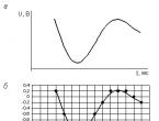
The solution can be illustrated by the diagram presented in Fig. 5, where D and S are the demand and supply curves, respectively, and the equilibrium position (with values And ) corresponds to their intersection point Q. The price at the initial moment of time is equal to P o . The corresponding point Q o on the curve S gives the volume of supply in period 1. This entire supplied volume of goods is sold out at a price P 1 given by point Q 1 on the curve D with the same ordinate (X 1) as Q o . In the second period of time, movement occurs first vertically from point Q 1 to a point on the curve S giving X 2, and then horizontally to point Q 2 on curve D. The last point characterizes P 2. Continuation of this process gives web graph, shown in Fig. 5. Prices and volumes (purchases - sales) in successive periods of time are respectively the coordinates of points Q 1, Q 2, Q 3,... on the demand curve D. In the case under consideration, the sequence of points tends to Q. In this case, the points are alternately located on to the left and right sides of Q. Consequently, the price values ​​P t tend to, located alternately on both sides of. The situation is exactly the same with the volumes of purchases and sales (X t).

The solution can be obtained algebraically for the case of linear supply and demand functions: D = a+ aP, S = b+ bP. Equilibrium values And will be given by the equations

A +a = b +b,

that is

= (a - b )/(b - a), = (b a - a b )/(b - a). (10.4) . p t-1. (10.7)

Equations (10.7) are similar to (10.5), except that they describe deviations from equilibrium levels (it is now known that such exist). Both of these equations are first order difference equations. Let us set c = b /a and substitute it into equation (10.7), so that the difference equation is relative R t will

R t = c p t-1 . (10.8)

At this value R o at the moment t = 0 from (10.8) we obtain the solution:

R t = R o c t,

or

P t = + (P o - ) c t .

Equation of the form

where some numbers are called a linear difference equation with constant coefficients.

Usually, instead of equation (1), an equation is considered that is obtained from (1) by passing from finite differences to the value of the function, i.e., an equation of the form

If there is a function in equation (2), then such an equation is called homogeneous.

Consider the homogeneous equation

The theory of linear difference equations is similar to the theory of linear differential equations.

Theorem 1.

If the functions are solutions to the homogeneous equation (3), then the function

is also a solution to equation (3).

Proof.

Let's substitute the functions in (3)

since the function is a solution to equation (3).

Lattice functions are called linearly dependent if there are numbers such that and at least one is different from zero, for any n the following is true:

(4)

If (4) occurs only when then the functions are called linearly independent.

Any k linearly independent solutions to equation (3) form a fundamental system of solutions.

Let linearly independent solutions to equation (3), then

is a general solution to equation (3). When a specific condition is found, it is determined from the initial conditions

We will look for a solution to equation (3) in the form:

Let's substitute into equation (3)

Let's divide equation (5) by

Characteristic equation. (6)

Let us assume that (6) has only simple roots It is easy to verify that are linearly independent. The general solution of the homogeneous equation (3) has the form

Example.

Consider the equation

The characteristic equation has the form

The solution has the form

Let the root have multiplicity r. This root corresponds to the solution

If we assume that the remaining roots are not multiples, then the general solution to equation (3) has the form

Let us consider the general solution of the inhomogeneous equation (2).

A particular solution to the inhomogeneous equation (2), then the general solution

LECTURE 16

Lecture outline

1. The concept of D and Z - transformations.

2. Scope of application of D and Z - transformations.

3. Inverse D and Z transformations.

DISCRETE LAPLACE TRANSFORM.

Z – CONVERSION.

In applied research related to the use of lattice functions, the discrete Laplace transform (D - transform) and Z - transform are widely used. By analogy with the usual Laplace transform, the discrete transform is given in the form

where (1)

Symbolically, D - the transformation is written in the form

For offset trellis functions

where is the offset.

Z – transformation is obtained from D – transformation by substitution and is given by the relation

(3)

For a shifted function

A function is called original if

2) there is a growth indicator, i.e. there are such and that

(4)

The smallest number (or the limit to which the smallest number tends) for which inequality (4) is true is called the abscissa of absolute convergence and is denoted

Theorem.

If the function is original, then the image is defined in the domain Re p > and is an analytic function in this domain.

Let us show that for Re p > series (1) converges absolutely. We have

since the indicated amount is the sum of the terms of a decreasing geometric progression with the indicator It is known that such a progression converges. The value can be taken to be arbitrarily close to the value , i.e., the first part of the theorem is proven.

We accept the second part of the theorem without proof.

The image is a periodic function with an imaginary period

When studying an image, there is no point in considering it on the entire complex plane; it is enough to limit the study to any strip of width. Usually, a strip is used on the complex plane, which is called the main one. That. We can assume that the images are defined in the half-strip

and is an analytic function in this half-strip.

Let us find the domain of definition and analyticity of the function F(z) by setting . Let us show that the semi-strip plane p is transformed by transformation into a region on the z plane: .

Indeed, the segment , limiting the semi-strip on the plane p, is translated on the plane z into the neighborhood: .

Let us denote by the line into which the transformation takes the segment . Then

Neighborhood.

That. Z – transformation F(z) is defined in the domain and is an analytical function in this domain.

The inverse D transformation allows one to reconstruct the lattice function from the image

(5)

Let us prove the validity of the equality.

Lie inside the neighborhood.

(7)

(8)

In equalities (7) and (8), residues are taken over all singular points of the function F(s).

The use of equations is widespread in our lives. They are used in many calculations, construction of structures and even sports. Man used equations in ancient times, and since then their use has only increased. A difference equation is an equation that connects the value of some unknown function at any point with its value at one or more points located at a certain interval from the given one. Example:

\[Г (z+1) = zГ(z)\]

For difference equations with constant coefficients, there are detailed methods for finding a solution in closed form. Inhomogeneous and homogeneous difference equations of the nth order are given, respectively, by equations where \ are constant coefficients.

Homogeneous difference equations.

Consider the nth order equation

\[(a_nE^n +a(n-1)E^n1 + \cdots +a_1E + a_1)y(k) = 0 \]

The proposed solution should be sought in the form:

where \ is a constant value to be determined. The type of proposed solution given by the equation is not the most common. Allowable values ​​of \ serve as the roots of the polynomial of \[ e^r.\] When\[ \beta = e^r \] the expected solution becomes:

where \[\beta\] is a constant value to be determined. Substituting the equation and taking into account \, we obtain the following characteristic equation:

Inhomogeneous difference equations. Method of undetermined coefficients. Let us consider the difference equation of the nth order

\[ (a_nEn +a_(n-1)En^-1+\cdots+ a_1E +a_1)y(k) =F(k) \]

The answer looks like this:

Where can I solve difference equations online?

You can solve the equation on our website https://site. The free online solver will allow you to solve online equations of any complexity in a matter of seconds. All you need to do is simply enter your data into the solver. You can also watch video instructions and learn how to solve the equation on our website. And if you still have questions, you can ask them in our VKontakte group http://vk.com/pocketteacher. Join our group, we are always happy to help you.